Final report for FS14-282
Project Information
1 - Background
First introduced into Louisiana in 1751, sugarcane (Saccharum officinarum) is the highest valued row-crop in the state. Its continuous production is an important historic and economic component of Louisiana's overall economy. While recent decades have seen a drop in Louisiana sugarcane acreage, crop values have remained stable due to increases in sucrose yield. Significant increases in yield are mainly attributable to the addition of nitrogen (N) fertilizer.
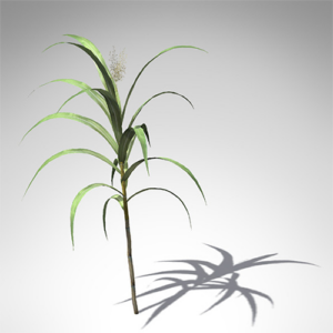
Figure 1. Saccharum officinarum (Sugarcane).
Problem
As the amount of harvested sugarcane declines, sugarcane growers in Louisiana are under pressure to boost their operational efficiency in order to sustain this economically vital crop. It is essential that producers apply new and proven technology in order to mitigate the cost of production, maximize yield, and limit impact on the environment.
Current Methods
Intensive agricultural production systems, like sugarcane, typically require a higher input rate of nitrogen (N) to achieve sufficient biomass and yield. Along with rate optimization the timing of N application is likewise important. Current methods employed to determine N status in sugarcane include visual inspection, tissue analysis, and chlorophyll monitoring. Soil analysis is used to gauge N content, but the reliability of sampling is inconclusive in the humid soils of southern Louisiana. Continuous refinement of effective and affordable N management systems is essential to maintain sustainable sugarcane agriculture in Louisiana.
The Value of Vegetation Indices
Our study considers the use of low-cost vegetation indices such as aerial NDVI as an addition to the overall N management scheme specific to sugarcane production in Louisiana. The Normative Difference Vegetation Index (NDVI) is a form of hyper-spectral imaging that collects and processes information across various wavelengths of the electromagnetic spectrum. In agriculture, the goal of NDVI imaging is to detect the relative strength of photosynthetic processes occurring in the field. While vegetation indices like NDVI have been applied in agriculture, the primary disadvantage of these methods has traditionally been their cost and complexity.
Study Goals
Our primary goal has been to determine to what extent low-cost aerial NDVI might be correlated with variable N rates applied to sugarcane. A secondary goal is to determine to what extent time-series analysis of low-cost NDVI imagery might be used to predict yield potential in sugarcane.
We asked two questions:
-
Can variable nitrogen rates applied to sugarcane be correlated with low-cost multi-spectral imagery?
-
Are models of acquired multi-spectral imagery predictive of sugarcane yield?
Access to Technology
Studies on Louisiana sugarcane growth indicate that remote sensing methods like NDVI may be effective in predicting sucrose yield in response to applied N fertilizer. Yet access to these technologies by farmers is limited; acquiring, processing and interpreting such data is costly and time-consuming. While high-resolution aerial imagery such as NDVI holds the potential to improve operational efficiency, economic factors prevent their general adoption by Louisiana sugarcane growers.
High temporal and spatial resolution NDVI can provide a host of potential uses in agriculture in addition: prescribing N fertilizer amounts and estimating crop yield are two of the potential benefits to Louisiana sugarcane producers. Yet a 'chicken and egg' problem exists in allocating time and resources necessary for technology that has yet to be been proven in the field. Our study intends to make these tools available, in order to refine and measure their effectiveness.
Our report provides background and results of a two-year study on the feasibility of using different multi-spectral indices to predict sucrose yield in sugarcane. A goal has been to explore methods that are accessible in terms of cost and complexity when compared with traditional methods. We also offer guidance regarding the efficacy of the tools and methods considered.
Our report is organized into twelve sections. At the end of each section there is a link back to the Table of Contents.
- Introduction
- This document.
- Through the Eyes of a Plant
- An introduction to the biology of plant life.
- Background on Methods
- An overview of approaches used this study.
- Kites, Balloons, and Drones
- A description of low-cost aerial options available, their strengths and weaknesses.
- Varieties of Spectral Index
- A look at the kind of vegetation index used in this study.
- Pre-Processing Steps
- How raw image data were initially prepared.
- Post-Processing Steps
- How the image data were prepared for statistical analysis.
- Study Results I - Balloons and Kites
- Results when using balloons and kites.
- Study Results II - Aerial Drones
- Results when using Unassisted Autonomous Vehicles (UAVs), i.e. aerial drones.
- Summary
- What we've learned so far.
- Credits
- Credits and appreciation.
- References
- Comprehensive listing of resources used in this study.
Section 2 - Through the Eyes of a Plant
Basic Plant Biology
- Plants use chlorophyll, water, and carbon dioxide to synthesize sugars.
- Chloroplasts cells contain chlorophyll which absorbs light, mainly in Red and Blue wavelengths.
Our study sought to provide an assessment regarding the use of aerial imaging to determine the health and productivity of sugarcane. Before discussing our work, we first consider some basic principles of what such systems measure and how they achieve their results.
Photosynthesis is the process used by plants to synthesize sugar from carbon dioxide and water. The leaves of a plant contain photosynthetic engines known as chloroplasts. When sunlight hits these cells they absorb the Red and Blue wavelengths of light while reflecting away most others. Water, carbon dioxide, and filtered light produce sugars for the plant and oxygen for the environment.
Blue, Green, Red and Near Infra Red (NIR)
- Healthy plants absorb Red and Blue bands of light while reflecting away most of the NIR.
- Near infrared (NIR) light is generally damaging to plants.
Light visible to the human eye lies roughly between 380 and 750 nanometers (nm) along the electromagnetic spectrum. Plants are also receptive to light though the mechanisms involved are distinct from humans. The more healthy a plant is - i.e. the more photosynthesis it carries out - the more Red it tends to absorb. This behavior is correlated with the functional health of chloroplast cells as these are the drivers of photosynthesis.
If a plant's chloroplasts are damaged they will tend to absorb less Red light while reflecting away less near infrared (NIR). The ability to photosynthesize and produce sugar will likewise be diminished. Plants also absorb Blue, in fact they absorb more Blue than Red, however the rate of photosynthesis is higher in terms of the amount of Red absorbed.
In addition to absorbing Red (and Blue) and reflecting Green, healthy plants reflect away most of the NIR. NIR light is not visible to humans and neither may plants convert this higher energy form of light to useful work. It is in part to avoid the damage that NIR might otherwise cause that plants reflect most of it away.
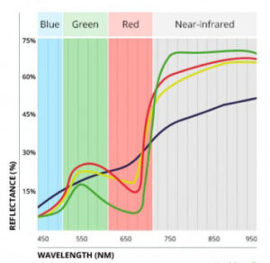
Figure 1. Spectral signature showing behavior of healthy (green), stressed (red), nitrogen deficient (yellow), and necrotic (purple).
In Figure 1 reflectance values are on the 'y' (vertical) axis while the wavelength of light is on the 'x' (horizontal) axis. In healthy plants Blue is largely absorbed and only a little is reflected. As we move into the Green the amount of reflectance increases. In the Red it is again diminished while in the NIR (the grey region) almost all is reflected away.
In addition to showing the 'spectral signature' of a generic plant this graph indicates important differences between healthy and unhealthy plants. The green line shows the reflectance profile of a healthy plant while the red line indicates a distressed one. Note that unhealthy plants absorb less in the Blue and Red while absorbing more (reflecting much less) in the NIR portion.
The spectral signature of sugarcane generally follows that of any other green leafy plant - it absorbs 60 to 85 percentage of incident light minus the Green band (most is reflected away, hence leaves appear green to us) and minus most of the NIR light. Sugarcane's outer leaf is nearly transparent to infrared light while its inner mesophyll scatters this radiation either upward (reflection) or downward (transmission).
In recent decades remote sensing technology has improved and use of multi-spectral imagery has become an effective tool in monitoring vegetation conditions. The goal in gathering multi-spectral imagery for crop monitoring is to use a camera with sufficient sensitivity in all bands of the spectrum. As the price of sensors has continued to drop the range of options has increased, sometimes dramatically.
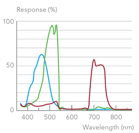
Figure 2. Spectral signature of a typical consumer-type RGB camera.
Figure 2 highlights the spectral characteristic of a generic consumer camera. The graph indicates that consumer cameras are sensitive in the Red, Green and Blue parts of the spectrum but not specifically in each narrow band, i.e. the RGB bands overlap. The 'width' of the Blue and Red bands is 100nm while the Green is somewhat less wide. Consumer cameras are not designed to separate each band of light which is acceptable in the context of taking consumer pictures. When the intended goal is to provide separation for purposes of quantifying luminosity values it's less than ideal.
Professional Multi-Spectral Cameras
- Multi-spectral cameras are tuned to capture multiple, narrow bands of light.
- The 'spectral signature' of a plant can help us understand its health and productivity.
Our study made use of consumer cameras as tools for gathering multi-spectral imagery with mixed results. An alternative to consumer-grade RGB cameras is a more expensive camera designed from the ground up to function as a true narrow-band instrument. Specialized multi-spectral cameras contain 'band-pass' filters which taper each wavelength of light. Gaining access to a narrower band in this way allows for more precise estimation of luminosity values.
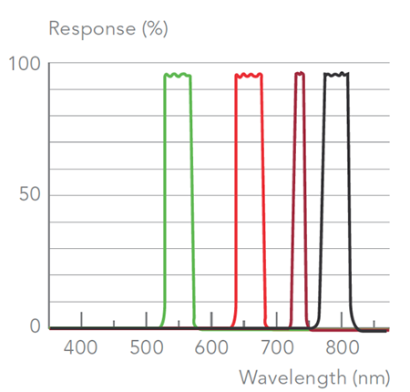
Figure 3. Narrow band spectral response of a Parrot Sequoia camera.
In Figure 3 the spectral response of a Parrot Sequoia camera is shown. With this camera Green is captured in the 530–570 nm band with peak absorption around 550 nm. The reflectance of Green is often correlated with leaf chlorophyll content. Variation in the Red band (660nm) often reflects changing attributes such as biomass, humidity and stress. Red reflectance also helps to distinguish plant from soil material.
Following Red is a very narrow band known as the Red Edge (730–740 nm). This band corresponds to the abrupt switch that occurs between Red and the higher reflectance values of NIR. An increase in Red Edge reflectance occurs often when a plant is experiencing nutrient stress.
The near infrared (NIR) band is captured in the 770-810 nm range. NIR is reflected away most when compared to the other bands and is sensitive to plant health and type. Since chlorophyll pigment does not influence NIR reflectance it is often used to 'normalize' the more chlorophyll-receptive bands. A drop in NIR reflectance indicates a plant under stress. The Red and NIR were the most extensively used bands in this study.
Summary
In the next section we discuss different types of multi-spectral camera used in this study and provide examples of each. We also discuss strategies for managing large volumes of data that are generated by this sort of workflow. It will become apparent that managing the data along with understanding how each vegetation index performs under changing environmental conditions presents certain challenges. Open-source software and image processing tools will be used throughout to make these tasks more tractable and accessible to the average user.
Section 3 - Background on Methods
Introduction
Here we provide a narrative description of the methods used to generate and assess multi-spectral data. This is not a typical 'Methods and Materials' section as might be found in a more traditional scientific paper. In Section 8 and Section 9 we go into more detail regarding our specific methods. Here we set the stage for what follows and describe some of the challenges faced and overcome.
One challenge relates to our project's having two opposing goals. On the one hand, we wanted to investigate low-cost methods in aerial photography for agriculture. This was motivated by personal interest along with a conviction that farmers have under-utilized available remote sensing technology, perhaps believing these were too complex or expensive. On the other hand, we wanted to answer questions that demand a level of precision regarding tools and methods. Exploring low-cost methods while seeking to answer empirical questions that demand accuracy (which comes at a cost) brings with it a certain tension. The questions posed by our study are presented in the Abstract but are re-stated here:
-
Can variable nitrogen rates applied to sugarcane be correlated with low-cost multi-spectral imagery?
-
Are models of acquired multi-spectral imagery predictive of sugarcane yield?
We were keen to answer these questions using methods which are accessible and available at modest cost. Our interest was to discover the types of vegetation index needed to correlate and predict sugarcane yield. One of these questions was correlative and we assumed it would surrender to whatever method we chose. The second question involved prediction and we thought it would be more difficult to answer unless the data captured was of high quality.
It turned out that neither question could be answered conclusively using the sort of flight and image capture systems that we originally proposed. The reasons will be addressed but in brief they are two-fold:
- Neither kites nor balloons are able to place a camera in position for sufficient time, under conditions of sufficiently stability, such that the results from one flight can be compared with results from another.
- While the sensors of a modified consumer camera are capable of capturing the right spectral data (i.e. the Red, Green and NIR light) the jpeg image format which most consumer cameras use does not support the sort of calibration necessary to quantitatively compare one day's flight image with another.
Our primary goal was to determine to what extent low-cost aerial multi-spectral data could be correlated with variable nitrogen rates applied to sugarcane. At the end of the first season we analyzed the data and came to the conclusion that the methods proposed would not work. Around the same time a third method became available that previously had seemed out of reach owing to its cost and complexity.
Creating the Right Spectral Index
An effective spectral index is built in stages by capturing light of the right band, at the right time of day, during the right part of the season. During our study it became apparent that the ability to place a camera in reproducible position for sufficient periods was the determining factor regarding whether our data could serve for more than qualitative assessments. Likewise, it became clear that the ability to capture in the narrowest band possible with minimum distortion was crucial.
A vegetation index can be created using only a single consumer digital camera as all consumer sensors are sensitive in the near infrared range. If the camera is modified to remove the IR blocking filter and a dual band pass filter is substituted (such that one channel captures visible light and either of the other two captures NIR) this leaves either the Green or the Blue channel available to capture NIR. However, in this scenario selecting which of the Blue or Green channel to use has an impact on the index and neither is likely to generate a result comparable to another taken on a different day. An improved solution is to use a dual-camera system where one camera captures Red while another captures the NIR. In such systems band pass filters are used to narrow the Red and NIR bands captured so that there is less contamination between them.
As an example of a dual-camera system, the composite in Figure 1 represents an RGB/NIR pair in the top row (left/right) captured with a pair of consumer digital cameras. The NIR photo on the top-right was taken using a modified Canon A590, from which the internal IR block filter has been removed. This sequence was created by Dr. Chris Fastie, a collaborator on this project.
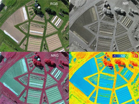
Figure 1. A composite image containing RGB (top left), NIR (top right), NGR (CIR composite, bottom left), and NDVI renderings.
In the bottom row (Figure 1) two images are displayed after post-processing. On the left a false color IR image (also known as a CIR composite) contains varying degrees of Red that represent the near infrared band. In the right is a 'normalized difference vegetation index' NDVI image which was created using the pair above. In Section 8 and Section 9 we will take a closer look at results obtained using these and similar methods.
Normative Difference Vegetation Index (NDVI)
NDVI is a popular vegetation index which has been shown effective in predicting crop yield potentials in other plant species. The expression used to create an NDVI index is (NIR - Red) ÷ (NIR + Red). This expression says subtract the Red band of light from the NIR band (in the numerator) add the Red band to the NIR (in the denominator) find the quotient between the two. As an example, assume that the amount of Red reflected from a plant is 8% and the amount of NIR reflected is 50%. We'd have the following NDVI expression:
(0.5 - 0.08)/(0.5 + 0.08) = 0.42/0.58 = 0.72
An NDVI of 0.72 (on a scale of 0 to 1.0) indicates that the plant is doing well. It reflects 8% of the Red away while absorbing the remaining 92% for photosynthesis. It also reflects more than half of the harmful NIR. This is a generic pattern that we will use: higher NDVI values correlate with healthier, more productive plants. Consider the same equation applied to a different plant:
(0.4 - 0.3)/(0.4 + 0.3) = 0.1/0.7 = 0.14
Compared with the first example, this plant is doing poorly. An NDVI of 0.14 indicates that it absorbs more of the NIR light while reflecting away a good portion of the Red. Recall that plants use the Red band to power photosynthesis while NIR light presents a physiological burden. This is another generic spectral pattern that we will use: lower NDVI values correlate with unhealthy, distressed plants.
Creating Larger Images
NDVI is only one, albeit important, vegetation index that was used in this study. In Section 5 we discuss other index types and their specific advantages. But before creating the index itself the images must first be captured and retrieved.
Whether one uses a kite, a balloon, a drone, or a pidgeon for image capture, once the images have been taken and the craft returned safely to ground, all images must be gathered together and 'stitched' to create a final representation. Figure 3 shows the result of stitching a dozen or so images from a balloon flight. This task is commonly performed by software but here an application provided by the citizen science group Public Lab is used to visually stitch each image over a map of the areal extent. This approach reveals how an image is often stretched and distorted in order to make it fit orthogonally onto a planar map. Achieving a seamless result requires exact overlap with identical exposure times between images.
The resolution of the image data gathered and stitched together ultimately rests on a number of factors, each representing a point in the overall process where error may be introduced. The ultimate goal of stitching images is to form a reflectance map - a mosaic of the area of interest where each pixel in the image represents the reflectance of the imaged area.
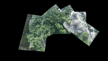
Figure 2. An animation of the stitching process. A dozen images are manually brought together into one larger image.
In turn, the resolution of the final image depends on the stability of the capture event, the resolution of the camera, and the stitching process. Of interest is the resolution per pixel. With regard to aerial photography, resolution (also called ground sample distance) refers to the area of ground covered by an individual pixel. With regard to a digital camera, resolution can also refer to the number of pixels contained in the sensor. When using the term 'resolution' we usually mean the ground sample distance. This important concept is covered in greater detail in Section 8 when discussing the results of kites and balloons.
Interpreting Spectral Indices
We have seen that interpreting a vegetation index starts with acquiring accurate aerial image data and that doing so requires consideration of two fundamental issues:
-
Placing the camera at the correct height and orientation for a sufficient period of time.
- In Section 4 three possible methods for positioning a camera in the air (a kite, a helium-filled balloon, and an aerial drone) will be considered. Each has its advantages and disadvantages.
-
Acquiring sufficient spectral detail from a camera such that the data may be usefully analyzed.
- The phrase 'sufficient spectral detail' will be unpacked but essentially means clear separation of the individual bands of captured light.
Figure 3 illustrates a typical NDVI result using a kite-suspension system with two consumer-grade cameras modified for NDVI. The image in the center of the figure represents a color LUT (i.e. a look-up table) which is used to apply a color transform to an image. Applying this transform allows us to visualize reflected light that otherwise would be impossible to see.
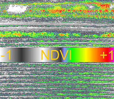
Figure 3. An NDVI index image taken with a consumer grade dual-camera system. The center bar is a color LUT.
In the image the LUT is prominently displayed in order to indicate that a full range of values has been captured in this image - from dry, sandy soils on the upper left (with an NDVI value of -1) to active areas of photosynthesis on the upper right. Also visible are regions of immature crop that are less well developed on the lower left compared with lower right.
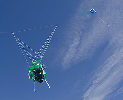
Figure 4. A dual camera system used to take the image contained in Figure 3.
Though it offers a qualitative view only, an index image produced from a kite remains a useful tool to help identify and track potential trouble spots in a developing crop. Having a simple kite rig in the back of the truck can assist in crop scouting. With a clear sky and brisk wind, a kite flight takes thirty minutes and is time well spent if it points out regions of the field that are underdeveloped or damaged.
While the result produced in Figure 3 is useful and may be achieved for a couple hundred dollars and a weekend of practice, these are qualitative, not quantitative results. If the goal is to measure patterns over time then this method will not work. While not impossible, it is difficult to replicate the exact height and vantage point of a image taken during a flight with a kite or a balloon. On another day under different skies such images will be hard to replicate. Since a stated goal was to use low-cost methods to accurately determine crop trends over time we decided to look for a more accurate solution.
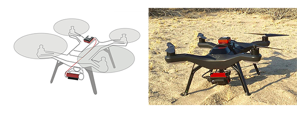
Figure 5. The 3DR Solo drone with a Parrot Sequoia camera and its 'sun sensor' (on top).
Semi-Autonomous Methods
Unmanned Aerial Vehicle (UAV) is an all-encompassing term which includes the aircraft, ground-based controller, and system of communication between the two. Commonly known as drones, semi-autonomous aircraft have been around for years but only recently have become available on the consumer market. The challenge of earlier drones in agriculture relates to their usability and cost. Prior to 2014 a fixed wing drone capable of flying (with payload) more than a few hundred yards cost anywhere from $10–30K. Small, high-resolution sensors were also available but these could add another $15-35K. Until recently it could cost anywhere from $25K to $65K to place a UAV in the air and retrieve meaningful data. Since 2014 that price has fallen to below $5000.00.

Figure 6. A multi-spectral narrow band camera, the Sequoia, produced by Parrot. On the right is the Sunshine sensor.
As UAV drone prices have fallen so too have options become available regarding use of a truly professional grade instrument (in place of a consumer camera). A Washington state-based company named Micasense produced the first small form-factor multi-spectral camera, the Sequoia, in 2016. Though the price of this instrument is high relative to a modified consumer camera, it is not out of reach. With Micasense's help we were able to use the Sequoia during the 2017 season.
The Sequoia is the same size as a GoPro camera. It's small and lightweight enough to serve as payload for a consumer-style drone such as the 3DR Solo. The camera includes a 'sun sensor' which sits on top of the drone (the camera is below pointing down).
Figure 7. A sugarcane field reflects light in specific ways that are picked up by the Sequoia camera, calibration occurs in tandem with the sunshine sensor.
Figure 7 indicates the value of the Sequoia compared with other cameras that we tried. The most troublesome aspect of a consumer camera (as discussed in Section 4) is the difficulty of calibrating each image such that the final stitched product contains uniform pixel intensities that accurately reflect the intensity of light during a particular flight. Calibration is crucial both within flight (since many images are stitched together) and between flights (since illuminant conditions change from day to day). If the intensity of light varies from moment to moment or from day to day, the amount of reflected energy from the field will be altered and the result will be innaccurate.
To manage the variability of light the Sequoia uses a 'sunshine sensor' to continuously record ambient light conditions in the same spectral bands as the camera sensor does. This ingenious system allows the camera to be used in clear or overcast conditions on the same day. Each image can be adjusted accordingly on-the-fly. This improvement was key to allowing us to record image data in a consistent and repeatable manner.
Summary
After an initial year of ups and downs using systems originally proposed it became apparent that for a modest investment one could use an aerial drone instead. Our team was among the first to fly a 3DR Solo drone with the Sequoia camera.
Various flying methods, while interesting in themselves, are only a means to the end of placing a camera into position in order to capture the right light at the right time of day. Before venturing into the core methods used in our study and the results obtained we first set the stage by discussing some earlier methods that were used and why they did not succeed.
For agricultural purposes, the broadband sensors contained in a modified camera are suited to a qualitative 'big picture' views of a crop's current status. However, the information provided by such cameras is limited and does not permit detailed analysis of a crop over time.
In the next we discuss the various bands of reflected and captured light and how these are used to facilitate our understanding of crop health. In Section 5 we consider in greater detail how such principles allow us to manipulate the captured bands and reveal more interesting and specific patterns. Here we have focused on general principles which makes all of this possible. More detailed results from balloon and kite methods are presented in Section 8 and in Section 9.
Section 4 - Kites, Balloons, and Drones
Introduction
- The goal in aerial data capture is to produce consistent, stable images.
- Cameras in flight are inherently unstable.
The history of taking photos from high-flying objects is long and storied, involving blimps, balloons, parachutes, kites, pigeons and personal drones. All these and more have been set aloft with ingenious cameras attached and tools to trigger them either remotely or automatically. The French caricaturist Gaspard-Félix Tournachon (known as 'Nadar') was first to fly and photograph the city of Paris from above in 1858.

Figure 1. Gaspard-Félix Tournachon hangs on, makes history.
Whatever method is used the object remains the same: position the camera at sufficient height, point it downward (as close to nadir as possible), get the shots, return the rig safely to the ground. None of the methods discussed in our report performed perfectly in all respects considered.
Let's Go Fly a Kite
- In certain conditions kites are incredibly stable and will fly for extended periods.
- Kites are easy to understand. Most people have flown one.
The image in Figure 2 shows a camera being suspended from a kite using a device known as a Picavet (named for French inventor Pierre Picavet). The Picavet attaches the camera to the line that flies the kite and holds it more or less in place. A Picavet consists of a rigid cross suspended below the kite line from two points.
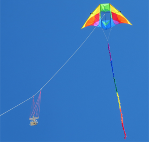
Figure 2. A camera system suspended via Picavet from a Delta-style kite.
Kites represent an easy and accessible solution to suspending cameras in flight and almost everyone has had some experience with them. Given a strong and stable enough wind a flying kite may be tied off and will remain suspended in the air for long periods without attention. On the other hand, while a Picavet is capable of orienting the angle of a camera roughly down, they don't prevent a camera from being jostled about during flight. In the event of a change in speed or direction the result may be blurred images mixed with a few good captures. Another consideration is the amount of effort required to retrieve a high-flying kite when facing a stiff wind. For kite-flying a pair of heavy leather gloves is always recommended!
Balloons
- Balloons serve as an alternative to kites on windless days.
- Helium is an expensive and non-renewable resource.
Figure 3 shows a 2-meter wide polyethelene balloon filled with helium gas. It uses a Picavet from which it suspends a dual-camera system similar to the one shown for the kite. The main difference between balloons and kites is in how each flies. Depending on size and payload (i.e. the weight of the camera plus the suspension system) a kite requires a sustained wind to become airborne. During this study our kite rig consisted of a 12' Delta-style suspending nearly half a pound of camera and triggering gear. Getting this rig into the air required a minimum sustained wind of 8-10 mph. On the other hand a helium balloon is sensitive and will be guided off course by a light wind. On a windless day the balloon rises easily to great altitude and remains steady in place for extended periods.
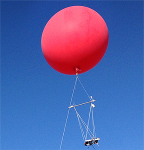
Figure 3. A helium-filled balloon suspends a dual-camera system.
We have found balloons and kites to be very practical and complimentary tools for aerial photography in agriculture. On windless days a helium balloon performs well while on a blustery one a kite is the better choice. In either case weather is key. The caveat of never putting into the air anything you aren't prepared to lose holds special meaning with either but especially with a balloon. While a kite will eventually descend, if you lose control of a balloon it will continue ascending and may drift into areas where it doesn't belong (i.e. into an airport's flight path).
A more practical concern regarding helium-filled balloons is that the element is in short supply. In some areas of the world helium use is restricted to essential medical and research purposes. Shortage in helium supplies has led to a rise in the cost of this lighter-than-air gas. One should consider this when deciding on helium use for non-critical purposes. While helium is naturally released from fossil-fuel production sites and may be captured and stored, after use it eventually escapes into space forever.
Unmanned Aerial Vehicles (i.e. Drones)
- Aerial drones (UAVs) are unique among the other methods discussed.
- UAVs provide stability and reproducibility over individual flights.
A recent development in aerial photography addresses some of the weaknesses found in other methods tried. While a UAV is technically an aircraft without a human pilot in fact all aerial drones rely on human direction. Perhaps it's more accurate to say that drones act semi-autonomously while being piloted remotely. Either way, they represent a significant improvement over other methods discussed.
Several attributes make UAVs unique among other methods. Chief among these is the ability to receive a pre-programmed flight plan where the height and extent of every mission is reproducible from one flight to the next. As we will see in later sections, this capability is especially important in the context of precision agriculture.
Aerial drone prices have dropped but owning and operating one remains an substantial expense. While a number of turnkey services provide all-in-one flight and data services, as in any new endeavor, understanding the steps involved and the actual value-add is crucial for success.
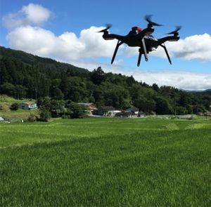
Figure 4. A 3DR Solo drone in mid-flight. The Solo drone was used in this study.
Here are some ways that aerial drone technology is being applied in agriculture:
- Soil and Field Analysis
- UAVs can be used at the start of a crop cycle to produce 3D maps. After planting, soil and field analysis maps can help direct irrigation and nitrogen-application.
- Planting
- Planting systems directed by UAVs can achieve higher uptake rates and lower overall planting costs.
- Crop Spraying
- With ranging technologies such as LiDAR drones can be used to apply the correct amount of liquid fertilizer or pesticide to the ground for even coverage.
- Crop Monitoring
- How to scale an effective crop monitoring plan remains an issue for most farmers. Satellite imagery has been used for large-scale crop monitoring but these data can be imprecise and are often expensive. Time-series data from successive UAV flights can show the development of a crop much more effectively.
- Health Assessment
- With UAVs it is possible to scan a crop in the visible and near-infrared bands and identify which areas are healthy or unhealthy. Vegetation indices can be used to track changes in crop health over time.
The goals of our study limits discussion to the last two categories (i.e. to monitoring and assessment of the health of a crop) however these and other developments like them have created a kind of revolution in agricultural science and practice. When we began this study the autonomous drone was a figment, its use in agriculture was limited and largely theoretical. UAVs were not a viable option unless one had very deep pockets and a background in aviation. Since that time UAVs have quickly evolved and become firmly established as a new norm in agriculture.
Summary
Small and large growers alike can benefit from the steep reduction in price and complexity of UAVs and multi-spectral cameras. Using such tools growers can acquire valuable forms of data as required and suit them to their specific needs. In addition to drones and precision cameras we also used kites, balloons, along with single and dual camera systems. Each has its place in agriculture and taken together all represent a leveling force of technology which holds the potential to assist small and medium-sized growers in farming more precisely and sustainably.
Section 5 - Varieties of Spectral Index
What's A Vegetation Index?
- A multi-spectral index is an expression relating bands of light as they reflect from an object.
- Narrow bands of light energy reflect from plants and inanimate objects in distinct ways.
There are a hundred different ways to create a spectral index, all sharing the property of representing a ratio where bands of light are manipulated in the numerator or denominator of a simple mathematical expression. Generating and interpreting a vegetation index (a spectral index applied to vegetation) provides a reliable way to compare a plant's photosynthetic activity and structural variation over time and space. A common spectral index used in agriculture for gauging the health of plants is NDVI ('Normalized Difference Vegetation Index'.)
Calculating a Vegetation Index
Calculating a vegetation index requires converting an image or set of images into a set of rasters - rectangular grids of pixels or points of color. Each pixel contains a set of values corresponding to the captured bands of light. In familiar RGB terms each pixel contains a Red, a Green and a Blue score. Such scores reflect the power, or luminosity, of electromagnetic radiation for that particular band as it comes into contact with the sensors of the digital camera. Most of the indices used in this study make use of an inverse relationship between Red and near infra-Red reflectance values commonly associated with healthy green vegetation.
Figure 1. Vector versus raster image.
An example vegetation index is NDVI which is calculated from an image in the following way:
- Subtract the NIR band reflectance values in all pixels from all the Red values.
- Add all NIR values in each pixel to all the Red values.
- Calculate the ratio between the calculated difference (the numerator) and the calculated sum (the denominator).
Performing the above calculations creates a third pixel value for every input pixel.
Calculating NDVI requires creating and manipulating separate images (i.e. pixel arrays) one of which contains light from the Red band and the other from the NIR band. The index is a ratio of differences and sums of these two narrow bands calculated separately over many individual pixel points. A ratio is taken in order to normalize values with the effect that this binds them between -1 and 1. Plant NDVI values can range from 0 to 1 but usually lie somewhere between 0.2 and 0.8.
![]()
Figure 2. Fastie LUT (Look Up Table)
Human eyes cannot see NIR light (or the ratio of differences and sums of NIR and Red) thus the final result must be 'colorized' in some way to have it make visual sense. The image in Figure 2 is a color 'LUT' or look up table that we use throughout the study to accomplish this. (For those interested in the RGB values used to create this LUT they are included in spectral_lib.py)
![]()
Figure 3. Scaling up an NDVI-processed section of the study area. The final image is a raster where each pixel represents a distinct reflectance value.
The image displayed in Figure 3 gives an idea of how coloring each pixel works. A more detailed description comes in Section 7 and Section 9. Here a portion of one section showing three rows of early growth sugarcane has been imaged as NDVI and colored using the color LUT described above. The range of NDVI values goes from low 'soil' to higher areas of growth. While an entire section is 412 by 72 pixels (100 x 20 ft) on the left part of Figure 3 only a portion of the full section is visible. The middle image shows more detail. On the right individual pixels are visible, each with a ground resolution of 2.7 centimeters (i.e. each pixel corresponds to a ground coverage area of about 1 square inch).
In summary, each pixel of the final vegetation index has a value representing a number between 0 and 1 and this represents a known area covering the ground. The strength of the NDVI value is used to infer a physical property, in this case the relative amount of photosynthesis occurring at that specific point. NDVI and other index values are 'dimensionless' meaning that the physical values from which they originate cancel one another out. In other words NDVI and other forms of vegetation index do not purport to measure a actual physical quantity. At best they only infer one. Common vegetation indices that were explored during our study include:
- NDVI = (NIR - Red) / (NIR + Red)
- The workhorse of vegetation indices, NDVI reveals the physical basis of most other VI's (i.e. the relationship between absorbed/reflected amounts of Red and NIR light). In our study, NDVI was best at revealing biomass differences. It was most effective in the early to mid-growth part of the season. NDVI tended to lose some sensitivity in the later season following canopy closure.
- SAVI = (NIR - Red) / (NIR + Red + L) * (1 * L)
- The soil-adjusted vegetation index (SAVI) is a modification of NDVI intended to correct for soil brightness. In areas where soil is exposed reflectance of light is altered in the Red and NIR bands and this may influence the final result. The issue is mainly present during the early part of the growth season. We addressed this through use of a custom masking technique discussed in Section 7.
- OSAVI = (NIR - Red) / (NIR + Red + 0.16)
- OSAVI is derived from the Soil Adjusted Vegetation Index (SAVI) above. It's sensitive to canopy density but not to soil brightness. Where vegetation cover is > 50% it may help dampen the saturation effect that NDVI is prone to. We used this index in the latter part of the 2017 season with mixed results.
- NDRE = (NIR - RE) / (NIR + RE)
- NDRE is available only in cameras that are sensitive to the 'Red Edge' spectral band. It's a better general indicator of plant health for mid to late season growth when compared to NDVI. NDRE is also thought to be capable of mapping variability in foliar Nitrogen levels, which we were interested in. Green and Red-edge bands penetrate the leafy part of the plant more so than the Blue or Red bands. Thus Red-edge is more sensitive to chlorophyll content and to nitrogen contained in the leaf.
- GNDVI = (NIR - Green) / (NIR + Green)
- As indicated by the name, the Green Normalized Difference Vegetation Index is related to NDVI (also sometimes called RNDVI) in that it uses the Green band while NDVI uses the Red. GNDVI is an index of 'greenness' and by that measure is more sensitive to photosynthetic activity, specifically to variation of chlorophyll content in plants.
- CIR Composite (Color Infrared)
- Unlike the other values described a CIR Composite is not a true index. Instead of displaying the common RGB bands it combines the NIR, Red, and Green bands such that the NIR is shown as Red, the Red as Green, and the Green as Blue. This allows the NIR light to be visualized as Red. We used CIR composite images extensively.
Choosing an Index for Sugarcane
- A healthy plant has a distinct 'spectral signature' based on unique reflectance properties.
- The spectral signature of a sugarcane field is a 'sum' of the total number of individual sugarcane plants.
The percent reflectance of any feature (i.e. water, sand, sugarcane) on the ground can be plotted to produce a spectral signature. Differences among spectral signatures are used to analyze and classify remotely sensed objects.
As discussed in Section 2, the spectral signature of sugarcane generally follows that of any other leafy green plant - it absorbs 60-85 percent of the incident light minus the Green band (most of this is reflected away, hence leaves appear Green) and minus most of the NIR light.
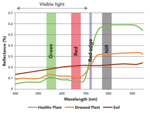
Figure 4. The spectral reflectance characteristics of healthy versus stressed sugarcane.
Like other leafy plants, sugarcane preferentially absorbs the Red band for photosynthesis. In Figure 2 all spectral lines (except for soil) reveal a characteristic bump in the Green band relative to the Red, indicating that Green is reflected away. In the right-hand portion of the curve nearly all of the NIR light is reflected away.
Sugarcane's spongy mesophyll is nearly transparent to infrared radiation thus very little NIR is reflected by the outer portion of the leaf. Mesophyll tissue and cavities within the leaf scatter most of the NIR light either upward (reflection) or downward (transmission).
Thus, depending on environmental conditions sugarcane will reflect light in distinct ways. These 'signatures' can reveal important information about different stages of growth or at different levels of photosynthesis.
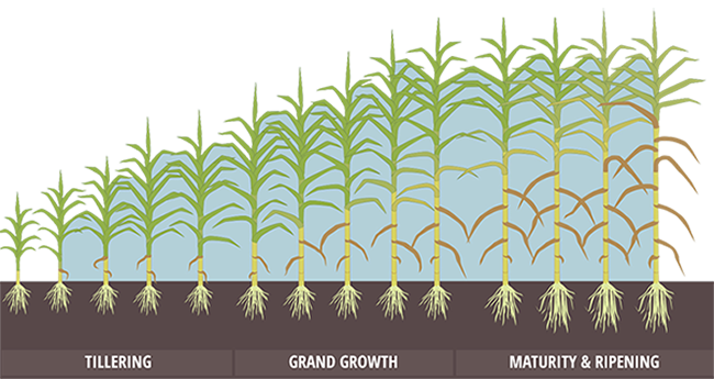
Figure 5. Stages of sugarcane growth that formed the focus of our study.
Sugarcane growth was monitored in our study in terms of a subset of the vegetation indices listed above (NDVI, GNDVI, NDRE, 'corrected' NDVI, and the CIR composite) at days 6, 21, 36, 100, 147, and 208 following nitrogen treatment. These times correspond to the shaded portions of Figure 5, i.e. they occur during the tillering, grand growth and maturation phases of the season.
Sugarcane is a perennial crop that grows to ~4 meters in height (in Louisiana) with a very high rate of photosynthesis (~150-200% above other species) as it rapidly progresses from tillering to grand growth.
Summary
To produce a vegetation index a narrow band of light (for example the NIR) is contained in one layer while another band (the Red) is held in another. By manipulating each pixel of each layer according to a mathematical expression, we produce a third raster layer which is the index layer itself. All of this is accomplished using software designed to perform matrix arithmetic over large pixel arrays.
While we've discussed simple calculations applied to single pixels, in practice generating a vegetative index over a crop involves much more. In addition to separate individual bands as arrays we need to scale these sorts of manipulations up to potentially millions and millions of pixels covering hundreds and hundreds of megabytes of image data. In coming sections we'll discuss how to achieve this degree of scaling. Luckily, open-source software and image processing tools exist to make these tasks accessible.
Section 6 - Pre-Processing Spectral Imagery
Introduction
This section describes various software tools and methodologies used to take raw captured images and transform them into a multi-spectral index suitable for statistical analysis.
Pre-Processing Steps
- Defining the initial processing steps.
- Quality control and reproducibility.
The automated system designed and implemented during this project performed a total of six processing steps. The first four are required to prepare the raw image data before it may be analyzed. The fifth and sixth are post-processing steps that are considered in Section 7.
- Mosaicking
- Atmospheric correction
- Geometric correction
- Image registration
- Masking
- Extraction of image-derived statistics
While proprietary software exists and may be used to implement the listed steps, the expense of licensing and training for such use is often prohibitive. The increased capability of open-source software to process multi-spectral data presents an opportunity for individuals and small teams to develop workflows for image processing that can be adapted when the need arises for little or no cost.
Mosaicking
Mosaicking is the process of taking two or more raster datasets (i.e. images) and combining them into a single, seamless image. Mosaicking can be accomplished using open-source applications such as QGIS, GDAL, or the Orfeo Toolbox. In our case several scripts based on GDAL were developed to accomplish a number of tasks, such as extracting metadata from uploaded images, handling cases where overlapped image pixels conflicted, or managing the map coordinate system.
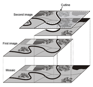
Figure 1. Creating a mosaic of several images.
Atmospheric Corrections
As the atmosphere intervenes between sun and ground it may distort the spectral distribution of light as it impinges upon the Earth. In the past, acquisition of spectral imagery was mainly limited to that acquired from aircraft or satellite, where the intervening distances are much larger. A key advantage of drones is that they fly close to their targets and thus atmospheric effects are minimized.
An atmospheric effect that cannot be mitigated with a drone is partial occlusion of light due to cloud cover. This happens not as one might expect, where there is consistent coverage, but rather where there's a patch of meandering cumulus passing in and out of the camera's frame. In this circumstance the delicate balance of calibration can be suddenly lost. An otherwise perfect day's flight may be compromised by a single pesky cloud.
Geometric Corrections
When aerial images are used in agriculture each feature of each image must accurately represent a true and consistent position on the ground. For purposes of this study the requirement carries weight since the tolerance for error is low. Achieving this level of precision requires both planimetric consistency (in the x,y orientation) as well as height invariance (in the z orientation). A high bar on flight stability is required since each location in an image must be translated into a standard geographical coordinate system representing the Earth's surface.
Aerial photography in the flat, alluvial deltas of southern Louisiana enjoys the benefit of relative stability in the 'Z' orientation. Here there are no sloping hills. In other situations (see Figure 2) ortho-rectification is critical where changing elevation may skew the accurate position of a point with its corresponding point on the ground. Nevertheless, in our case geo-rectification of images was still required and was facilitated through the use of ground control points (GCPs).
In addition, ortho-rectification is required to correct for image distortion arising from anomalies in the nadir positioning of the camera. Each time a drone doubles-back to cover another section it loses nadir position (the perpendicular aspect) with respect to the ground. It may also lose nadir at any point in the flight on a windy day. In either case, the necessary geometric corrections were performed using scripts that make use of GDAL functionality.
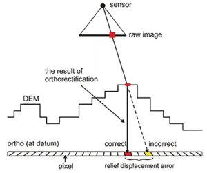
Figure 2. Orthorectification using a digital elevation model (DEM).
Image Co-Registration
One of two goals in our study was to consider the evolution of a spectral index over time as a way of making predictions about sucrose yield. When the intention is to study two or more images in a time series then image co-registration is required. Co-registration ensures that an image captured one day is spatially-aligned with an image of the same extent captured on another day. We were able to meet these criteria through use of GCPs and by having an area dedicated exclusively for the purposes of our study during the study period.
Another scenario where co-registration arises is when more than a single camera lens is used to capture images of the same object. Both the modified consumer camera and the Sequoia camera use multiple lens. In a workflow defined for the Sequoia camera we performed 'band-to-band' image alignment (a form or co-registration) in order to account for the distortion effects of multiple lens.
Summary
Nearly zero man-made infrastructure was present in our study area thus the images generated throughout were dependent for alignment on invariant structures occupying known positions in the field. In addition, we set up ground control points based on known latitude and longitude coordinates and on elevations. There was a very mild down-slope from one end of our study area to the other of about 0.5 meters
Section 7 - Post-Processing Spectral Imagery
Introduction
This section describes the tools and methods that were used to generate and interpret statistics from multi-spectral index images. These and other post-processing steps have formed a large part of our exploration of available methods for understanding the relationship between a given spectral index and the final sucrose yield in sugarcane.
While a number of technical details are discussed we hope to present them in a manner that remains accessible to non-technical users. A primary goal of this study is to provide information and access to methods for working farmers. While there will always be specialized knowledge, much of this work is accessible, more so than might first appear. It's an under-appreciated fact that growers are, as a rule, adept at picking up a new technology when it serves a practical purpose.
Open Source Automation Tools
- A range of open source tools are available to assist in processing multi-spectral imagery.
- Automation of the processing steps is both possible and desirable using open source models.
Our study made use of a number of software tools and libraries that are freely available as open source projects. Among other things, 'open-source' means that installing, learning and using these software products is open to anyone who has an interest. There are no licensing fees. In the context of this project all tools described have been applied during the study and new code continues to be added on a daily basis to our Github project repository. We have drawn on the strength of open-source tools in order to implement many pre- and post-processing steps. In fact, even the drone used in the study runs a stripped-down version of the open-source Linux operating system, i.e. one may login, get a command prompt, and execute code on the drone.
Post-Processing Steps
In any part of a multi-step process looms the spectre of error. This is especially true if the process relies on manual execution of a number of steps. In every phase of this project we have sought to minimize error by automating as much of the work as possible. The processing system designed for our project consists of six automated steps. The first four are required to prepare the raw image data prior to analysis and are covered in in Section 6. The fifth and sixth are post-processing steps that were subsequently performed. In this section we consider these final steps: masking and extraction of image-derived statistics.
- Mosaicking
- Atmospheric correction
- Geometric correction
- Image co-registration
- Masking
- Extraction of image-derived statistics.
Practical Examples
- Different spectral indices offer alternate views of the same data.
- Seasonal variation in spectral data can be addressed through basic machine learning techniques.
We tested a variety of spectral index types during our study, always with the goal of discovering which was best suited to the task of revealing an elusive set of values.
One question we sought to answer was how interaction of NIR light with soil effects the spectral index of an early sugarcane crop. Figure 1 below shows a pair of early season NDVI images, one taken in late April and one from late May. Nitrogen treatments for this crop occurred on April 19, 2017. The two images are significant insofar as they reveal the initial response to treatment and the sensitivity of a specific index in capturing it. Each image is an NDVI of the same section over time following application of 80 lbs N per acre. The first was taken 6 days after N application and serves as a baseline. The second is one month later in the season.
It turns out that this is a typical task in post-processing spectral data. We want to analyze image pairs in order to derive a better sense of the sensitivity of a particular index, and to correlate the average index of each pair. However, at least half of the visible area in these images is composed of soil which should not be included in the averaged NDVI value (e.g. soil is not photosynthetic).
Thus the task is to remove pixels from an image where those pixel values represent soil. How might one accomplish this? One way is to open up each image in an editor, examine every pixel and guess, based on color, whether it should be included in the final average or not. Each of these particular section images contains ~30,000 pixels and there are 30 sections in each dataset. That's roughly 900,000 pixel decisions to make for each.
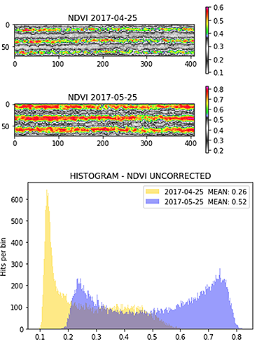
Figure 1. Histogram of soil-uncorrected NDVI values.
Instead of counting pixels, another approach is to look more closely at how the two images stack-up. To do this we can plot them as 'dual' histograms, as is done in Figure 2 below. Note that there are multiple peaks in each histogram (one is colored yellow and the other purple). The yellow peak at far left is the most prominent. This peak indicates that 'soil' pixels have an average NDVI value between 0.1 and 0.2. There are also peaks found in the purple histogram, corresponding to NDVI values from the 05/25 image, though these are not as prominent as the 04/25 image.
Masking
Examining the histogram of 'uncorrected' NDVI values in Figure 2 we see that the mean NDVI value for 04/25 and 05/25 is 0.26 and 0.52, respectively. These averages include the soil pixels in addition to the plant material. We can use the same data that generates the histogram as input into a type of 'classification' machine learning algorithm known as minimum threshold. This algorithm assumes that the image contains two pixel classes (foreground and background) which are used to calculate an optimum threshold to separate the two. In plain English this means that by applying the algorithm we're automatically masking the more prevalent pixel type (in this case the non-photosynthetic pixels) in a manner that is repeatable, i.e. not solely based on individual judgement.
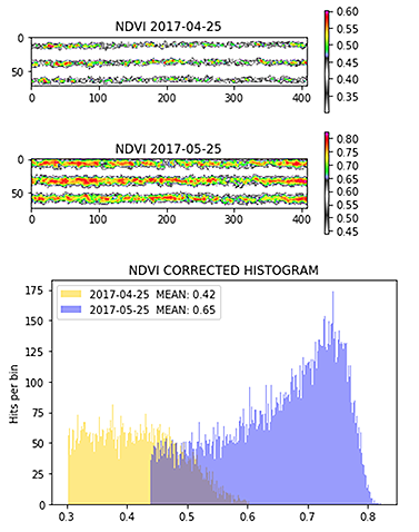
Figure 2. Histogram of 'corrected' NDVI values.
The result of applying minimum threshold is seen in a second set of images and in a histogram generated from the 'thresholded' data (see Figure 3). No longer do we see the prominent peaks (the 'soil' pixels are replaced by 'neutral' white). The second set of averages more accurately reflects the actual NDVI value of the crop, minus the noise. These values (in the 'corrected' versions for 04/25 and 05/25) are 0.42 and 0.65, respectively.
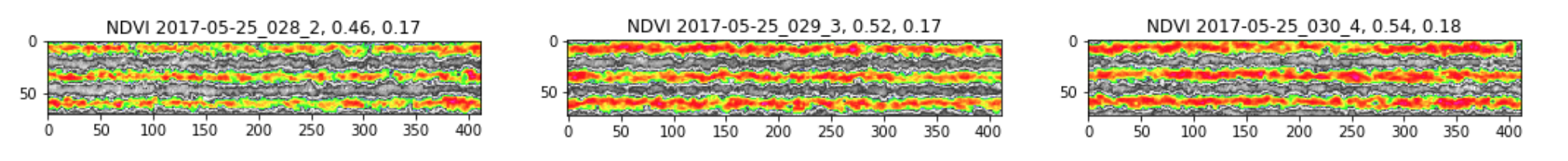
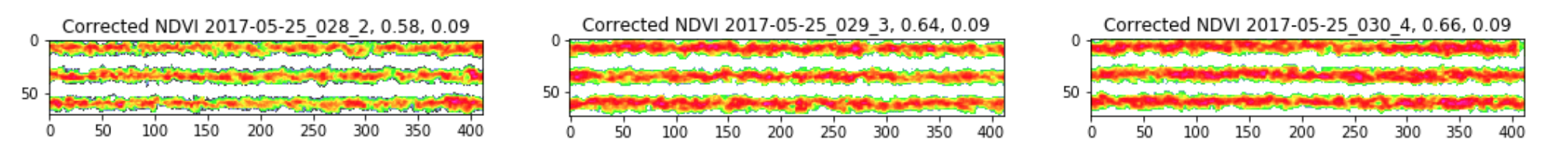
Figure 3. Set of soil corrected and uncorrected NDVI images.
This simple method illustrates how automating a single step in the chain reduces error overall. Figure 3 shows a set of three uncorrected/corrected NDVI images from May 25, 2017. The nitrogen treatments are, from left to right, 40 lbs N, 80 lbs N and 120lbs N. In the top row the unbiased standard deviations are 0.17, 0.17, and 0.18, respectively, while in the corrected versions they are 0.9 in each case. Here we've managed to remove some of the 'noise' from the samples which is significant when a final interpretation of these data is made.
Extraction of Image-Derived Statistics
- High resolution section images were used to create each vegetation index.
- Statistical analysis was performed on the vegetation index images.
Figure 4 below compares two NDVI images taken early in the growth season, at Day 6 following treatment and at Day 21. Section images like these were used as input to the statistical analysis and are the final word on our reported results. The specific images here are 412 by 72 pixels in size, where each pixel has a ground resolution of 2.7 centimeters (~1 square inch). These data were captured at a height of 250 ft while flying the drone at a speed of 10 mph. A single image capture occurred each second and comprised a set of RGB, Green, Red, Red Edge, and NIR images.
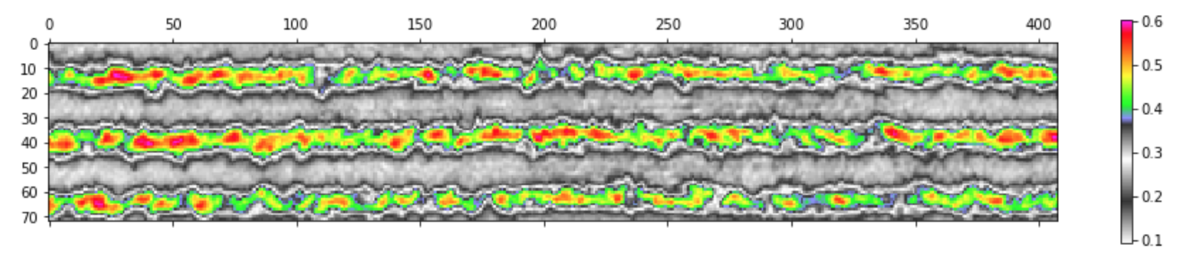
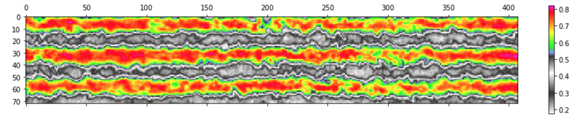
Figure 4. Comparison of NDVI images from April 25, 2017 and May 25, 2017.
The images in Figure 5 below demonstrate subtle differences when using an alternative vegetation index at a different point in the growth season. Two groups of nine sections are displayed one on top of the other. The top group is NDVI, the bottom is GNDVI. Reading each from left to right advances time from early season to the high point of photosynthetic activity. Reading them from top to bottom shows an increase in nitrogen treatment from 80 lbs N to 180 lbs N.
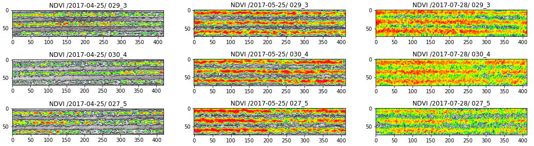
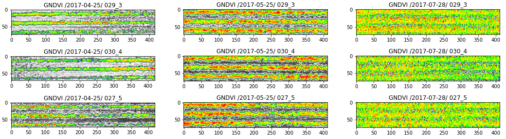
Figure 5. General comparison of NDVI versus GNDVI performance in early to mid-season sugarcane.
When analysed statistically these image data reveal that, compared with NDVI, GNDVI shows a lower correlation with yield data overall but may be better suited at certain points in the season. As indicated by the leftmost column, use of the Green band in sparsely vegetated sections decreases the sensitivity of GNDVI while denser sections (right-most column) tend to benefit by dampening the saturation that occurs with NDVI later in the season. Surprisingly, the central column is where GNDVI out-performs NDVI in terms of its ability to correlate with the final yield values.
Quality Control
An issue faced by this study and others like it is the relatively small number of samples produced, along with distortions due to error that any one sample may accrue before reaching the analysis phase. Our 1.5 acre test area contained 30 section plots with five treatments each, i.e. six samples for each date flown. Half of the flight data yielded inconsistent results and was therefore rejected.
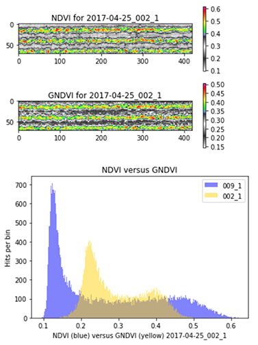
Figure 6. Comparison of different index types in the same section, same treatment.
For those data which we felt were acceptable we then imposed an additional set of criteria regarding what an index image needed to have in order to be considered 'finally' suitable. Our criteria included running various statistical analyses on different index types taken in the same section and/or treatment. For example, while the images in Figure 6 have not yet been soil-corrected they reveal a characteristic relationship between GNDVI and NDVI where the former has less energy i.e. it displays fewer hits per bin across the entire reflectance range and those hits are more 'bunched' together around a central mean value.
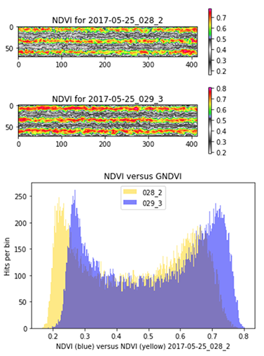
Figure 7. Comparison of the same index for different sections, similar treatments.
In a similar way we can compare index images from different sections using the same index to measure a similar treatment. The treatments in Figure 7 are for 40 lbs N (yellow) and 80 lbs N (Blue). The NDVI values that make up this histogram are for sections imaged on the same day (the same flight) at Day 36 following treatment. What we expect to see is a characteristic shift to the right of the plot receiving the higher treatment and this is what we do see.
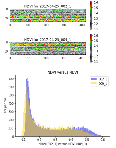
Figure 8. Comparison of the same index for different sections, same treatment.
The last sort of comparison we did, as a means of 'proofing' whether or not an image sample was acceptable, was to check different sections with the same treatment. In Figure 8 two NDVI images that received 0 lbs N in different parts of the field have similar (not identical) histogram plots.
Summary
This section might raise a legitimate concern among some that we have pre-selected data that was most likely to submit to a favorable analysis. Indeed there is a tension between cleaning data so as to removes outliers and 'null' values (which is acceptable) and removing meaningful information. A guiding principle of this study has been to reveal whether or not certain low-cost methods were amenable to a certain kind of rigor. Getting a half dozen consistent datasets was a challenge for this study and it was thought that given what we set out to achieve special care should be paid to knowing whether or not the data were accurate prior to analysis.
In the next two sections we consider the results obtained by using various flight and capture methods. It will become apparent where accuracy is lost due to the piling on of error over steps in a longer process where ample opportunity exists for unintended mishap to occur.
Section 8 - Results Using Balloons and Kites
Introduction
When our project began the plan was to use methods that are readily available to anyone and to apply these in ways that do not impose a high barrier in terms of time and materials. Farmers are generally practical with regard to the kinds of tools they are willing to try. Most are eager to learn a new method if it helps solve a long-standing problem more efficiently.
As an example, crop scouting has existed as long as farming has and its methods have changed little except what was once done on foot or by horse is now done in a pick-up truck. If a kite and a camera can do the same work while adding more information then chances are these tools will be adopted. With that sentiment in mind we discuss results obtained by experimenting with kites and balloons
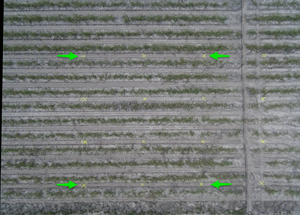
Figure 1. RGB image captured with a Delta kite at height of 125ft. Ground control points (in yellow) are visible.
Image capture and preparation
Figure 1 is a RGB composite image captured with a kite and stitched together 'by hand' with the help of ground control points (GCPs) spray-painted into the field. Having GCPs in a set of images like this is crucial both for stitching together the final image and for comparing image sets over time. To support this process we used an open source software known as Fiji. Fiji is an image processing package that bundles an incredible variety of plugins to facilitate scientific image analysis.
To determine the height of a flight we carefully measured and marked the kite's flight line. This set of captures was taken at a height of about 125ft. Maintaining a steady altitude like this with a kite can be a challenge when the wind is variable. This was a key challenge faced with kites.
JPEG versus RAW Format
In addition to challenges imposed by weather there are those associated with the choice of camera, especially the choice of image format. A common default for consumer cameras is JPEG (Joint Photographic Experts Group). The JPEG format in many cameras has processing built in at the time of capture, to adjust contrast, reduce noise or brighten and sharpen the image before rendering it to a file. These processing steps are intended to render images that are visually appealing to the human eye. As a result pixel values of a JPEG-processed image lack a 'true' relationship with the intensity of light that impinges on the sensor. Details regarding how a JPEG file is processed by a particular camera are not easy to come by and disabling such 'features' is usually not a practical option.
Other sources of artifact in JPEG images are compression and band distortion. Digital Image Compression (DIC) attempts to address the issue of storage and transmission since space is usually at a premium in a consumer-grade camera. For our purposes, image pre-processing, compression and band distortion are less features than issues to be corrected. They impact an ability to utilize all the bandwidth data in post-processing.
As an alternative, some consumer cameras support the RAW format, which preserves all of the bandwidth data. However, RAW images are larger than JPEGs and the rate of capture required during flight (to achieve an acceptable ground resolution) makes their use prohibitive. For this reason our results using consumer cameras are based on the JPEG format. How to accurately calibrate for reflectance under changing illuminant conditions while limited to JPEG is an issue that has been addressed by others (for excellent work in this area see Public Lab postings here and here).
Finally, the lack of accurate geo-tagging support in most consumer cameras means there's no reliable source of reference regarding planar or vertical positioning of the camera with respect to the ground. A hand-held GPS device was used to create the ground control points in these images but it was not always possible 'geo-tag' and match each capture with a known position on the ground. Having obtained a set of images we then scripted a process in Fiji to help align, stitch and create the vegetation index.
Post-processing JPEG images
Details regarding how to create a vegetation index such as NDVI using the Fiji software package are described in detail by Chris Fastie and Ned Horning on Public Lab's website here and here. The Public Lab community is a leader in this field and the information they have compiled over the years serves both as an inspiration and as a working guide throughout.
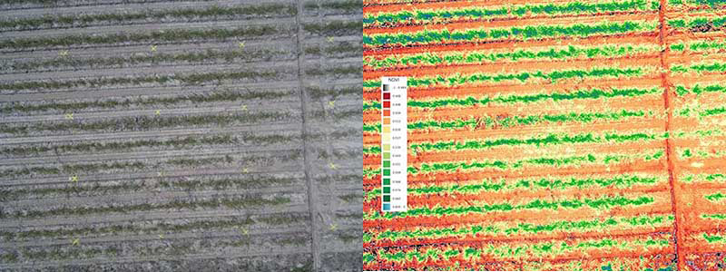
Figure 2. RGB and NDVI image processed using Fuji. The RGB image was captured with a Delta kite at a height of 125ft.
Figure 2 is an NDVI index derived from RGB and NIR sets using a pair of modified consumer cameras. It was taken from a height of about about 125 ft early in the growth season. The vertical LUT displays NDVI values between 0.45 and 0.60. This particular image shows an interesting effect that we saw throughout while using our dual-camera NDVI system. The NDVI values of soil show values in the lower range (0.45) compared to the green areas of early growth. At low altitude our dual-camera system tended to record non-vegetation sources lower than at higher altitudes while remaining fairly consistent overall in terms of vegetation.
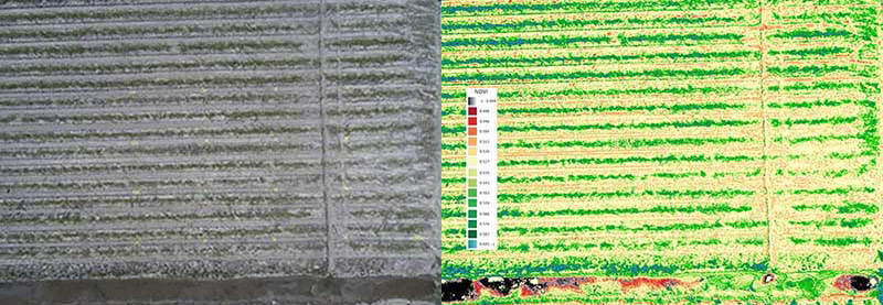
Figure 3. RGB and NDVI image from 200 ft.
Figure 3 is another NDVI index derived from RGB and NIR image sets, this time taken from a height of about 200 ft. The only difference between this figure and the one above it is an increase in altitude of 75 feet. Each image was taken on the same day with the same lighting conditions and in the same section of the field. Each was processed identically.
While we were able to understand and explain these and other anomalies the purpose of this report is not to delve into details but to make a recommendation regarding the methods explored. It was our experience that such deviations tended to accumulate and, in the end, left our results in question.
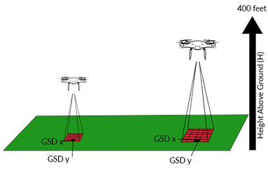
Figure 4. Relationship between height and ground sampling distance (GSD).
Various factors contribute to the overall resolution of an image taken from the air. Of interest is the ground sampling distance, i.e. the distance between pixel centers measured on the ground. Since a key advantage of a kite or balloon (or drone) is the ability to fly close to the ground we made an effort to understand exactly how improved GSD effects our results for sugarcane.
The resolution of satellite imagery is relevant as these methods demonstrate why other lower-cost method are desirable. Aerial imagery generated by satellite or airplane has traditionally been the only solution available to sugarcane farmers. A disadvantage of these methods is their cost and relatively low resolution. A key advantage is their wide coverage.
![]()
Figure 5. Relative pixel dimension depending on satellite image source provider.
The goal in aerial imaging is to get as high as possible without sacrificing resolution but the tension between the two factors can be complex.
For example, the GSD of a Landsat satellite image is ~30m (b. in Figure 5). This means that the smallest unit that maps to a single pixel in Landsat is 30m x 30m (900 sq m, 0.22 acres, ~8% of our total study area). Each of our thirty test sections measures 100ft by 20ft (a. in Figure 5) thus a single pixel in Landsat is five times larger than a single section.
While Landsat data is freely available commercial satellite providers charge for higher resolutions (e.g. providers like Planet Labs supply a GSD of 5 m, or a pixel size of roughly 250 sq ft, c. in Figure 5). The GeoEye-1 satellite offers the highest resolution at a little over 1 sq ft per pixel. In addition to cost and a generally lower GSD, delays between successive captures, cloud-cover, and other atmospheric effects can present significant challenges to a grower's reliance on satellite or airplane data service providers.
Minimum Resolution for Accuracy
All resolutions discussed thus far are for standard RGB imagery. For multi-spectral bands including NIR these resolutions drop slightly thus RGB alone is a higher resolution image when compared to all bands taken together. Our choice of a pair of Canon S100 consumer cameras meant a high pixel count and with flight altitudes between 100 and 200 ft we were confident, in principle, that our GSD was more than adequate. At these heights our GSD was from 3-5 sq in or between 0.06-0.17 sq ft per pixel. In Section 9 we discuss results achieved using an aerial drone where the attained ground resolution is 2.7 centimeters or about 1 inch square per pixel.
There are reasons to belabor the degree of resolution on the ground. During our study many other factors contributed to reduce overall resolution and impact the final result. Each step was a piece in the puzzle that ultimately decided whether the final result should be held up as a useful guide to decision-making. Initially it was our thought that results using a kite and a modified camera would get the last word but it turned out that these methods, while certainly useful, were themselves insufficient.
All of the methods considered in our study were explored and utilized for the same reason: to produce, at reasonable cost, a consistent set of image data that could be relied upon over time. Each in its own way does this. Satellites produce a wealth of image data that may be usefully mined. Kites and modified cameras are easy to make and deploy and the results obtained from using them are often startlingly rich in detail. In Section 9 we will see how the performance of aerial drones form a kind of sweet spot between the two.
Summary
Early in the project we experimented with various automatically-triggered cameras and suspension systems using kites and balloons. The central challenge of an aerial system based on wind alone is variability in the control of height and nadir positioning of the camera. Additional factors to consider are payload weight and total flight time.
Our results using a kite and a pair of modified consumer cameras were insufficiently consistent to be useful for the main study goals of the project. However, they are eminently well-suited for other purposes. Having a Delta kite and a single or dual camera rig ready in the back of one's pickup truck seems a no brainer for crop-scouting and general field intelligence work.
Section 9 - Results Using Drones
Introduction
- An area of second-year sugar cane 'stubble' measuring 1000 ft by 60 ft was dedicated during the 2017 year.
- A series of random sections were laid out and treated with variable amounts of nitrogen fertilizer.
Once planted, a stand of sugarcane may be harvested up to four times in as many seasons. In Louisiana, a season runs about 9 months and after each harvest the cane remaining in the ground sends up new shoots. While successive harvests yield decreasing amounts of sucrose, the crop used in this study (a second-year stubble) is an ideal 'nitrogen-absorber' and was thus well-suited.
For the 2017 season, a single-factor field trial was laid out in a common randomized split-plot design on 19 April 2017 (see Figure 1).
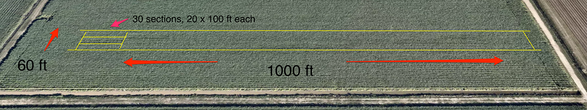
Figure 1. Ellendale study area measuring 1000 by 60 ft, 1.5 acres total.
As indicated in Figure 2 below five levels of nitrogen fertilization (0, 40, 80, 120 and 180 kg·N·ac−1) were applied in a setup with six replicates. This resulted in 30 plots of size 100 × 20 sq ft each making a total trial size of 1.5 acres.
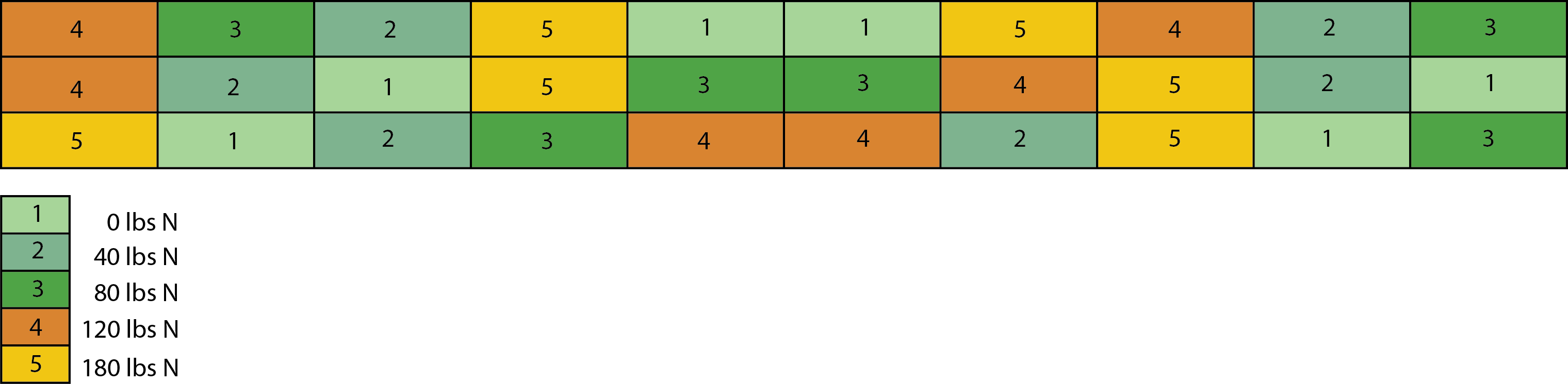
Figure 2. Treatment schedule applied during the 2017 sugarcane season.
Sugarcane growth was monitored at 6, 21, 36, 100, 147, and 203 days after N treatment (DAT). At 210 DAT the experimental plots were harvested and analysis of sucrose yields was performed. The yield was measured following manual harvest and weighing by means of load cells.
Drone flights were made over the area during the 2017 growth season on eleven separate occasions. Data from half of these flights were used in the analysis. The study area was flown and captured over two separate flights for each date (due to power consumption reasons) where each flight overlapped in the center of the field. Calibration of the Sequoia camera was performed between each flight.
A primary advantage of the drone compared with other methods is the ability to pre-program an exact height (250ft) and range prior to each flight. This advantage is clearly demonstrated in Figure 3 taken from 'nadir' perspective. It shows two 100 x 20 ft sections in perspective. As indicated here the precision offered by semi-autonomous, programmable drones outperforms other aerial methods considered.
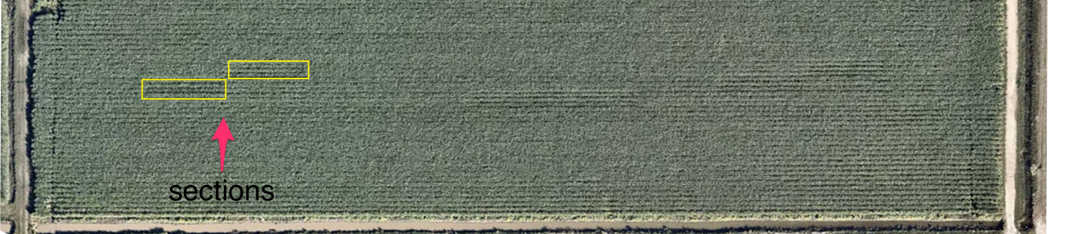
Figure 3. A 'nadir' view indicating the relative scale of individual sections.
Processing Steps
- After pre-processing, each flight yielded a single composite image.
- The composite was segmented by an automated process into the thirty individual sections.
- Statistical analyses was performed on each section in terms of four spectral indices.
To capture the study area each drone flight yielded roughly 1200-1500 geotiff images using the Sequoia camera. Raw single band images containing the four bands of light (plus RGB) were layered to produce from 300-350 composites. These composite images were then stitched together into a single master geotiff.
The process of stitching geo-coded images is known as mosaicking (see Section 6 ). Mosaiking allows accurate placement of acquired image data and projection of those data onto a map. The process was facilitated in this study by embedded latitude and longitude tags in each image captured by the Sequoia camera. This allows us to create images of relatively high definition containing a broader field of view.
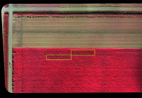
Figure 4. A detail of two treatment sections rendered as a CIR composite image.
The image in Figure 4 has been rendered as an CIR composite for visualization purposes. The original raw geotiff from which it was produced contains only luminosity data from the four bands of captured light. The original composite also contains geotags which form part of the image's metadata. One of the challenges of precision mapping is to correctly match a partial image - which may have been distorted in the process of capture - with an actual landmark on the ground.
The process of stitching is often facilitated through use of ground control points (GCPs). A GCP is an invariant point of reference on the ground that stitching software uses to better align corresponding points in an image. For our purposes this process was aided by use of a camera that accurately records and embeds latitude, longitude and elevation data in each image such that they are matched together in the final composite. GCP's referenced from a surveyor's benchmark were also used and were physically located in the ground.
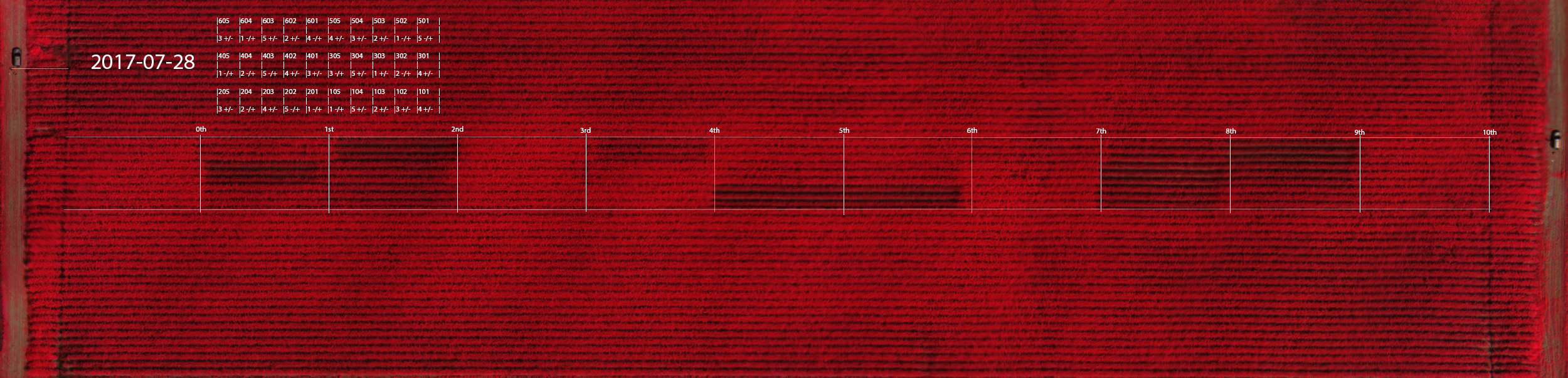
Figure 5. A CIR composite showing section detail over the entire study area. Color differences indicate different nitrogen treatments.
Figure 5 shows results of a flight which occurred on July 28, 2017. This image has been rendered as an CIR composite and clearly shows, as Red light, the conditional coloring of luminosities in the near infrared band. Also visible are differences in areas that have been treated with variable amounts of nitrogen.
Our treatment schedule for 2017 was 0 lbs N per acre, 40 lbs, 80 lbs, 120 lbs, and 180 lbs per acre. These amounts were chosen as they reflect a sensible range around the recommended treatment for this particular species (120 lbs per acre).
Comparing Plots
- Section treatments were analyzed during early, mid, and late-season growth.
- A cumulative ‘index signal’ for each section was derived as the mean of all pixel values.
Prior to analysis the master geotiff file for each date (containing precise coordinates of latitude and longitude) was sectioned to produce thirty consistent areas representing each treatment section. Sectioning was performed using an automated method guided by embedded latitude and longitude coordinates.
The development and growth of the leafy part of the sugarcane plant plays a role in helping to maximize the interception of solar energy for photosynthesis. This leads to the accumulation of biomass and ultimately to a higher crop yield. Our results indicate that sucrose yield was significantly improved by N fertilizer application. Compared to control the yields for the 2017 season for cultivars under 40, 80, 120 and 180 kg·N·ac−1 were 45%, 50%, 62%, and 55% higher, respectively. Our first successful data capture occurred just a week following N treatment.
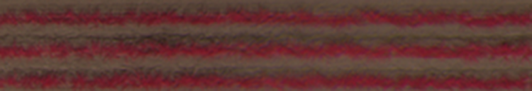

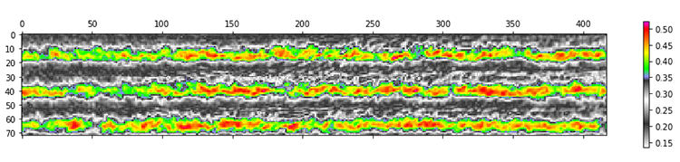
Figure 6. CIR composite image, NDVI versus GNDVI index in an early sugar cane crop.
In Figure 6 three images from early in the season are displayed: on top is a CIR composite of a single section (taken on April 25, 2017) followed by two index images below processed from the same section for NDVI and GNDVI. The color bars to the right represent index values on a scale of 0 to 1. The mean 'soil-corrected' index value for each section was 0.46 for NDVI and 0.4 for GNDVI. These values were generated for all sections, for all treatments, and used in the final regression analysis. Our approach was to average a cumulative 'index signal' for each section and then compare this with the final sucrose yield for that section following harvest.
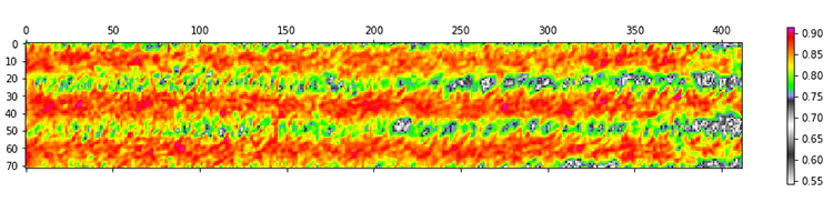
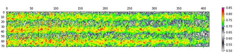
Figure 7. CIR composite image, NDVI versus GNDVI index in mid-season sugarcane growth.
In Figure 7 a CIR composite, NDVI and GNDVI from a section taken later in the season on July 28, 2017. The mean 'soil-corrected' index value for these was 0.83 for NDVI and 0.73 for GNDVI. Given the obvious visual difference of these two images, that the values are basically the same (after accounting for the scale difference) was of interest.
A Digression on Regression
Regression is a statistical technique used to estimate relationships among variables where focus is often put on a dependent variable along with one or more independent variables. The independent variable is the 'predictor' while the dependent variable is the quantity one hopes to predict. During our study a question was posed regarding whether two variables might be correlated with one another and to what degree. Another was asked regarding whether one variable might be predictive of the other.
There's a popular truism in statistics: 'correlation does not imply causation'. The saying carries with it a negative connotation, as if correlation were something of lesser value. When one finds a correlation between variables it can be tempting to say that there must be a causative relationship between the two. However, while we present evidence of correlation between vegetation index values and sucrose yield there is no causative element here (obviously the index didn't cause the sugarcane to form sucrose). Still, correlation and other measures of association can be useful for purposes of prediction irrespective of a causative connection.
Our 'dependent' variable was the amount of sucrose produced in each of thirty sections treated with a known level of nitrogen. The final yields (numbering 30) were measured in the lab at the end of the season and, along with our 'independent' variable, were known prior to analysis. The data were subjected to statistical analysis to determine the differences among treatments. Pearson correlation coefficients were calculated and regression analyses and models were built using Scipy and Pandas. All graphs were plotted with Matplotlib or Seaborn.
The graph in Figure 8 is a scatterplot of sixteen points each representing a single treatment. Each point is colored in terms of the treatment received by that section. On the 'x' axis are NDVI values and on the 'y' axis are 'pounds sucrose per section' (PSPS).
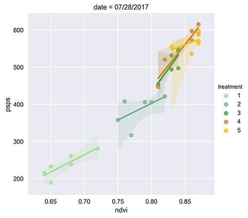
Figure 8. Scatterplot of a vegetation index (NDVI) versus sucrose yield, measured in pounds of sucrose per section (PSPS).
Earlier we spoke of the bugbear of cumulative error and that issue is no where more relevant than here in Figure 8. The values representing each data point (there are six per treatment group) are index values averaged over a set of ~30,000 pixels representing an area of 100 ft by 20 ft. The points of error that we have previously discussed (i.e. the accuracy of a camera's placement, the prevailing wind, sun angle, azimuth, and a hundred others) are embodied in every point in this graph. And yet in spite of this we see a very logical pattern of correlation. These data were captured on July 28, 2017 at the height of the grand growth phase. The index type shown is NDVI.
This single plot says less on its own than it does when compared with similar plots. However, viewed by itself it indicates that correlation between NDVI mean values and yield was strongest at 120 lbs N per acre (treatment #4). This is the recommended treatment for this variety of sugarcane. The degree of correlation is weaker for treatments both above and below this amount with the exception of 80 lbs per acre.
Multiple Regressions
The regressions that we have constructed for each index may also be compared in terms of their progression throughout the growing season. Figure 9 shows the progression of NDVI results from April 25th (six days following treatment) to November 13th (one week prior to harvest). Several points are of note: 1) plotted data moves from left to right in each graph as the season progresses, indicating a general rise in average NDVI values across all treatments; 2) the values of each treatment class 'spread out' as the season develops; and 3) the degree of correlation peaks at or around the height of the grand growth stage, after which it begins to fall apart. Of note is the consistently high degree of correlation between Treatment #4 (the recommended 120 lbs N per acre).
Figure 9. NDVI scatterplots from April 25, 2017 to November 13, 2017.
Animated Regression
To highlight the evolving nature of NDVI during the season Figure 10 animates the progression from April 25th to November 13th. Again several things are of note. At the start of the season (04/25) there is low correlation (R=0.39) among all treatment classes and sucrose yield. As the season progresses the correlation score rises and is visible in the graphic as a regression curve begins to tighten. At the height of the growing season the R value peaks of 0.97. Following this it then declines as the crop reaches maturation nearer to harvest.

Figure 10. Animated plot of correlation evolution between vegetation index (NDVI) and the yield produced by that section.
Faceted Regression
The results presented in Figures 8, 9 and 10 pertain to NDVI index values only. As part of our analysis we compiled similar statistics for other index types, including a 'corrected' form of NDVI, NDRE, and GNDVI. Figure 11 presents a 'facet' view of each of these and indicates the sort of index which performs best given a particular time in season.
Figure 11. Regression 'facets' showing index values versus yield (April to November 2017).
While the results in Figure 11 are qualitative it was our experience that the 'corrected' form of NDVI (top row) performed best early in the season (the red square highlights May 10th), the NDRE index (second from top) did best later in the season on November 13th, though it also did well very early on (April 25th). GNDVI (third row from top) tended to do best at the start of the grand growth phase likely due to canopy closure. Lastly, NDVI (bottom) was the overall winner and achieved the highest degree of correlation at the height of the grand growth phase. NDVI was the most consistent and highly correlated index throughout the majority of the season.
Temporal Evolution of Vegetation Index in Sugarcane
The results for NDVI and other index measurements versus sucrose indicate significant correlation during the 2017 season. The Pearson "r" values of each index type ranged differently during the year with NDVI showing the highest degree of correlation on July 28th, 2017 (100 DAT). The correlation coefficients of all four index types were relatively low in the early growth stages but achieved a robust relationship by about 100 DAT thereinafter.
Figures 12 through 15 show the degree of Pearson correlation of the four index types (corrected NDVI, NDRE, GNDVI, and NDVI) as the season moves from 6 days to 200 days following treatment.
Figure 12. Correlation of NDVI-C Index with Yield (measured as pounds sugar per section).
Figure 12 shows the temporal evolution of a 'soil-corrected' spectral index during the 2017 growing season. Correcting for soil effects early in the season results in an improvement over uncorrected values, but applying the same method later in the year following canopy closure reduces the degree of correlation. By the end of season there is no benefit in correcting for soil as it is no longer visible from above.
Figure 13. Correlation of NDRE Index with Yield (lbs sugar per section).
Figure 13 shows the temporal evolution of the NDRE index during the 2017 growing season. This vegetation index shows a wider dynamic range earlier in season and is sensitive to changes in the early crop. Since the Red band is more strongly absorbed by the top layers of the plant canopy an NDVI index is not as sensitive to the lower levels of the plant compared with NDRE. NDRE is also more sensitive in terms of its correlation with leaf area index (LAI) which is a variable we did not consider during our study. This effect increases in plants with more leaf layers such as a sugarcane crop in late stage growth.
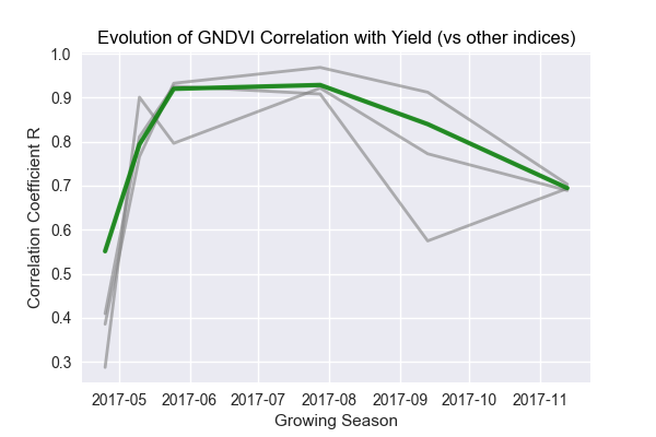
Figure 14. Correlation of GNDVI Index with Yield (lbs sugar per section).
Figure 14 shows the temporal evolution of the GNDVI spectral index during the 2017 growing season. GNDVI is a modified version of NDVI and is generally more sensitive to chlorophyll content. The chlorophyll content of the sugarcane leaf is highly correlated with nitrogen uptake.
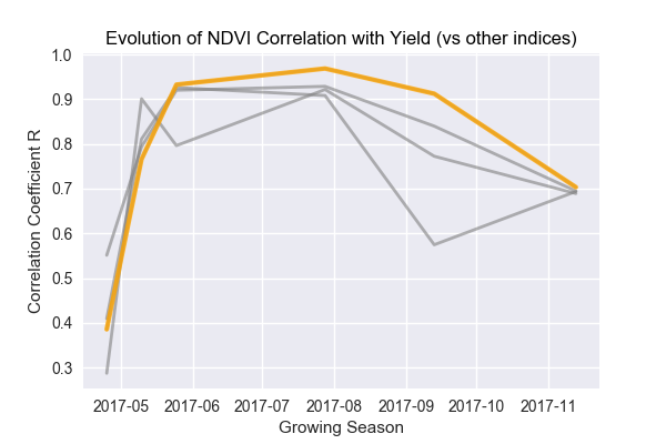
Figure 15. Correlation of NDVI Index with Yield (lbs sugar per section).
Figure 15 shows the temporal evolution of the NDVI spectral index during the 2017 growing season. NDVI attained the highest degree of correlation with sucrose yields over the different N treatments. NDVI's use in crop-yield estimation has been studied in other plant species. However, few studies have focused on yield estimation in sugarcane using high resolution techniques available at modest cost.
Summary
Results from the regression analyses indicate that the 100 DAT period is the most appropriate time for yield prediction of sugarcane using the NDVI index. We do not make the argument here but based on additional analysis we feel an exponential yield prediction model is likely the best fit (where the growing rate at around 100 DAT is in proportion to the remaining growth). Given the growth characteristic of sugarcane at the 100 DAT mark, an exponential model would be, we feel, most suitable for estimating the growth rate of sugarcane at this stage.
In our two-year study, the Pearson and regression analyses shown indicate that NDVI obtained at 100 DAT is significantly associated with the sucrose yield of this second-year variety of sugarcane. We feel that our methodology - using a low-cost consumer drone (the 3DR Solo) along with a Sequoia multi-spectral camera - represents an accurate and convenient toolset for determining in-season yield of sugarcane. This comparatively simple and low-cost method can provide an alternative approach for Louisiana sugarcane growers to estimate the yield potential of sugarcane while allowing for N management adjustments when necessary.
Section 10 - Summary
Achieving the highest possible sucrose yield at the lowest cost is the goal of every Louisiana sugarcane grower. To sustain sugarcane's viability Louisiana farmers must continuously seek new ways of boosting their operational efficiency while mitigating the costs of production. Tools and methods that were once prohibitively expensive and untested have become affordable and demonstrably effective in supplying information that addresses these goals.
Our two-year project employed remote-sensing and GIS technology to monitor crop performance and sucrose yield in south Louisiana sugarcane. In our report we have demonstrated that sucrose yield is strongly correlated with aerial NDVI measurements made at 100 days following treatment with nitrogen. Two different but related questions were investigated:
-
Can variable nitrogen rates applied to sugarcane be correlated with low-cost multi-spectral imagery?
-
Are models of acquired multi-spectral imagery predictive of sugarcane yield?
We feel that the first question has been answered. Indeed, applied variable nitrogen rates have been strongly correlated with each of several vegetation indices chosen for this study. The NDVI index was most effective overall but other types tested performed well under differing circumstances related to the time of season. These data were gathered and analyzed at very modest cost relative to comparable methods available.
An answer to the second question is pending further work but we feel that the methods used and the lessons learned over the period of our study provide ample evidence that predictive models based on vegetation index data alone are indeed possible. We are pursuing these questions in the up-coming 2018-2019 season.
A traditional limitation of remote sensing in agriculture has been its cost and complexity. Effective crop monitoring via aerial methods must be timely and of sufficient resolution. Neglecting issues related to its atmospheric effects the 30m resolution of non-commercial satellite imagery (Landsat 8) does not suffice for sugarcane. Higher resolution imagery from satellites (or airplanes) is available but these data are expensive and require pre- and post-processing to render them useful. The advancement of technologies such as UAVs and narrow-band image capture systems has brought us to a kind of tipping point.
There is a need for more reliable and actionable information that can assist Louisiana sugarcane farmers and other stakeholders in optimizing their operations. In addition to benefitting individual growers, the methods presented here are of use in helping to address the daily running costs incurred by a dwindling number of sugar mills that remain in south Louisiana. Better yield prediction data can make supply-chains between growers and refiners more efficient.
The use of remote sensing technologies to achieve yield estimates has been under-utilized by Louisiana sugarcane growers, in part due to cost and to the learning curve required. Here we have presented evidence indicating that NDVI obtained at 100 DAT is significantly associated with sucrose yield in sugarcane. Furthermore, these correlations may form the core of more predictive methods. These data were acquired using a drone and camera system of modest cost and by employing methods which we have published here and elsewhere.
Section 11 - Credits
- Gerald McCollam conceived and wrote the grant and the report, gathered the image data, carried out the statistical analysis, and contributed to design of the experimental plots.
- Slattery McCollam provided dedicated access to the study site for the grant period.
- Dr. Richard Johnson proposed the field trial’s design and helped with editorial contributions.
- Dr Chris Fastie designed the dual-camera harness system and provided research notes.
Section 12 - References
-
Abdel-Rahman,E., The application of remote sensing techniques to sugarcane (Saccharum spp. hybrid) production: A review of the literature. International Journal of Remote Sensing · July 2008 DOI: 10.1080/01431160701874603
-
Agustín Solano et al 2016 J. Processing Pipeline of Sugarcane Spectral Response to Characterize the Fallen Plants Phenomenon. Phys.: Conf. Ser. 705 012025 (https://doi.org/10.1088/1742-6596/705/1/012025).
-
Babar, M. A., Reynolds, M. P., Van Ginkel, M., Klatt, A. R., Raun, W. R., and Stone, M. L. (2006a). Spectral reflectance to estimate genetic variation for in season biomass, leaf chlorophyll, and canopy temperature in wheat. Crop Sci. 46, 1046–1057. doi: 10.2135/cropsci2005.0211
-
Ball, S. T., and Konzak, C. F. (1993). Relationship between grain yield and remotely-sensed data in wheat breeding experiments. Plant Breed. 110, 227–282. doi: 10.1111/j.1439-0523.1993.tb00590.x
-
Boote, K.J.; Jones, J.W.; Pickering, N.B. Potential uses and limitations of crop models. Agron. J. 1996, 88, 704–716.
-
Benvenuti, F., Weill, M Relationship between multi-spectral data and sugarcane crop yield. 2010 19th World Congress of Soil Science, Soil Solutions for a Changing World.
-
Caturegli, L.; Corniglia, M.; Gaetani, M.; Grossi, N.; Magni, S.; Migliazzi, M.; Angelini, L.; Mazzoncini, M.;
-
dos Santos Simoes, M., Rocha, J.V., Lamparelli, R. Orbital spectral variable, growth analysis and sugarcane yield. Sci. Agric. (Piracicaba, Braz.), v.66, n.4, p.451-461, July/August 2009.
-
Elvidge, C. D., and Chen, Z. (1995). Comparison of broad-band and narrow- band red and near-infrared vegetation indices. Remote Sens. Environ. 54, 38–48. doi: 10.1016/0034-4257(95)00132-K
-
Guilherme, M.S. Duft, D.G., Kölln, O.T., et.al. The potential for RGB images obtained using unmanned aerial vehicle to assess and predict yield in sugarcane fields, International Journal of Remote Sensing, DOI: 10.1080/01431161.2018.1448484 (2018).
-
Haboudane, D., Miller, J. R., Tremblay, N., Zarco-Tejada, P. J., and Dextraze, L. (2002). Integrated narrow-band vegetation indices for prediction of crop chlorophyll content for application to precision agriculture. Remote Sens. Environ. 81, 416–426. doi: 10.1016/S0034-4257(02)00018-4.
-
Huang J., Wang H., Dai Q, and Han D. 2014. Analysis of NDVI Data for Crop Identification and Yield Estimation. IEEE Journal of Selected Topics in Applied Earth Observations and Remote Sensing, 7, 4374–4384.
-
Hunt, E.R. Jr., Daughtry, C.S.T. What good are unmanned aircraft systems for agricultural remote sensing and precision agriculture?, International Journal of Remote Sensing, DOI: 10.1080/01431161.2017.1410300. (2017).
-
Hunt, E.R., Jr.; Hively, W.D.; Fujikawa, S.; Linden, D.; Daughtry, C.S.; McCarty, G. Acquisition of NIR-Green-Blue digital photographs from unmanned aircraft for crop monitoring. Remote Sens. 2010, 2, 290–305.
-
Jackson, R., and A. Huete. "Interpreting Vegetation Indices." Preventive Veterinary Medicine 11 (1991): 185-200.
-
Jensen T. 2013. Precision and Smart Technologies in Agriculture: Study Book. University of Southern Queensland, Faculty of Engineering and Surveying. 166 pp.
-
Jhan, J.P. Rau, N. Haalab Investigation of parallax issues for multi-lens multispectral camera band co-registration. Remote Sensing and Spatial Information Sciences, Volume XLII-2/W6, 2017
-
Li, Y., Chen, D., Walker, C. N., and Angus, J. F. (2010). Estimating the nitrogen status of crops using a digital camera. Field Crops Res. 118, 221–227. doi: 10.1016/j.fcr.2010.05.011
-
Mello, M.P., et.al. STARS: A new method for multitemporal remote sensing. IEEE Transactions on Geoscience and Remote Sensing (April, 2013), DOI: 10.1109/TGRS.2012.2215332.
-
Morel J., Todoroff P., Begue A., Bury A., Martine J., Petit M. 2014. Toward a Satellite-Based System of Sugarcane Yield Estimation and Forecasting in Smallholder Farming Conditions: A Case Study on Reunion Island. Remote Sensing Journal, 6, 6620–6635.
-
Motohka, T., K. N. Nasahara, H. Oguma, and S. Tsuchida. 2010. “Applicability of Green-Red Vegetation Index for Remote Sensing of Vegetation Phenology.” Remote Sensing 2 (10): 2369–2387. doi:10.3390/rs2102369.
-
N. A. Streck, J. G. Hanauer, L. F. Gabriel, T. C. Buske, and J. A. Langner, “Leaf development and growth of selected sugarcane clones in a subtropical environment,” Pesquisa Agropecuária Brasileira, vol. 45, no. 10, pp. 1049–1057, 2010.
-
Orych, A. Review of methods for determining the spatial resolution of UAV sensors. Remote Sensing and Spatial Information Sciences, Volume XL-1/W4, 2015.
-
Pinter, Jr., Paul J.; Hatfield, Jerry L.; Schepers, James S.; Barnes, Edward M.; Moran, M. Susan; Daughtry, Craig S.T.; Upchurch, Dan R. (2003). "Remote Sensing for Crop Management". Photogrammetric Engineering & Remote Sensing. 69 (6): 647–664. doi:10.14358/PERS.69.6.647. ISSN 0099-1112.
-
Prasad A.K., Chai L., Singh, R.P., and Kafatos M. 2006. Crop yield estimation model for Iowa using remote sensing and surface parameters. International Journal of Applied Earth Observation and Geoinformation, 8, 26-33.
-
Precision Agriculture for the Sugarcane Industry. excerpted from Precision and Smart Technologies in Agriculture: Study Book (Jensen 2013) ISBN: 978-0-949678-34-8 (www.sugarresearch.com.au).
-
Rahman M. and Robson A.J. 2016. A Novel Approach for Sugarcane Yield Prediction Using Landsat Time Series Imagery: A case Study on Bundaberg Region. Advances in Remote Sensing, 5, 93–102.
-
Ray, T. "A FAQ on Vegetation in Remote Sensing." http://www.yale.edu/ceo/Documentation/rsvegfaq.html, updated 13 October 1994. Accessed February 2014.
-
Samborski, S.M.; Tremblay, N.; Fallon, E. Strategies to make use of plant sensors-based diagnostic information for nitrogen recommendations. Agron. J. 2009, 101, 800–816.
-
Steven, M., et al. "Intercalibration of Vegetation Indices from Different Sensor Systems." Remote Sensing of Environment 88 (2003): 412-422.
-
Silvestri, N.; Fontanelli, M.; et al. Unmanned aerial vehicle to estimate nitrogen status of turfgrasses. PLoS ONE 2016, 11, e0158268.
-
Wang, Y., Wang, D.J., Zhang, G., Wang, J. Estimating nitrogen status of rice using the image segmentation of G-R thresholding method. Field Crops Res. 2013, 149, 33–39.
-
Zhang, C.; Kovacs, J.M. The application of small unmanned aerial systems for precision agriculture: A review. Precis. Agric. 2012, 13, 693–712.
Image Sources
Section 1
Figure 1 image source: https://gamaya.com/wp-content/themes/gamaya/images/sugarcane-banner.jpg (used with permission)
Section 2
Figure 1 image source: https://gamaya.com/blog-post/hyperspectral-imaging-in-agriculture/ (used with permission).
Figure 2 image source: https://www.micasense.com/ (used with permission).
Figure 3 image source: https://www.micasense.com/ (used with permission).
Section 4
Figure 1 image source: https://en.wikipedia.org/wiki/Nadar (Brooklyn Museum, no known copyright restrictions).
Figure 2 image source: Ron Marcisak https://www.flickr.com/photos/ronskap/13173764143/in/pool-kaprigs/ (used with permission).
Figure 3 image source: Alan McConchie https://www.flickr.com/photos/almccon/ (used with permission) .
Figure 4 image source: Sam Pepple, Sample Cartography (used with permission)
Figure 5 image source: Chris Fastie, Courtesy of the [Public Lab](https://publiclab.org/), (used with permission).
Section 5
Figure 1 image source: https://www.micasense.com/ (used with permission).
Figure 2 image source: https://gamaya.com/wp-content/themes/gamaya/images/sugarcane-banner.jpg (used with permission)
Figure 3 image source: https://gamaya.com/blog-post/hyperspectral-imaging-in-agriculture/. (used with permission)
Section 6
Figure 1 image source: http://www.pcigeomatics.com/geomatica-help/COMMON/concepts/Mosaic_explainMosaicking.html (used with permission).
Figure 2 image source: http://www.pcigeomatics.com/geomatica-help/COMMON/concepts/Ortho_explainRigorous.html (used with permission).
Cooperators
Research
For discussion of the materials and methods please see our full report in the Project Objectives section.
For discussion of the results please see our full report in the Project Objectives section.
Educational & Outreach Activities
Participation summary:
The educational outreach component of this work will occur in the Fall and Winter of 2018.
Learning Outcomes
Project Outcomes
A goal of this study has been to assess the feasibility of methods used that are not generally available to farmers without hiring a 3rd party consultant. The ability of being able to quickly and accurately access nitrogen placement in the field without dependency on a 3rd party service can impart a unique benefit to the farmer.
For discussion of the Project Outcomes please see the full report in the Project Objectives section.
Our final recommendations are forthcoming.