Final report for GNC21-319
Project Information
Soil Health Indicators in Areas Affected by Pipeline Installation
In the US, approximately 2.5 million km of hazardous liquid pipelines and natural gas mains have been installed (PHMSA, 2021). Assuming a mean width for a pipeline’s right of way (ROW) of 30 m, affected areas represent approximately 7.5 million hectares. The installation of the Dakota Access Pipeline (DAPL) in 2016 created a cross-section of disturbed soil from northwest to southeast Iowa. Since that time, farmers have observed lower crop yields along the path of the pipeline and have implemented a variety of management practices to address that issue. This situation creates a unique opportunity to study the effect of pipeline installation on soil health indicators. To date, studies conducted on the effects of pipeline installation on
individual fields have observed that soil bulk density and pH tend to be increased, corresponding to a decrease in total porosity, water holding capacity, and organic carbon (Naeth et al., 1987; Soon et al., 2000; Yu et al., 2009; Antille et al., 2014; Tekeste et al., 2018). In the present study, previous work is expanded upon by stratifying soil samples by soil landscape position, management practice, and disturbed versus undisturbed areas. The pipeline path was divided into three parts: pile area, trench area, and traffic area. Samples collected every 30 cm to a depth of 90 cm were measured for nitrate, organic matter, available phosphorous, exchangeable potassium, magnesium, calcium and hydrogen, pH, buffer index, cation exchange capacity (CEC), percentage of base saturation of cation elements and texture. For hydrologic properties, one ring of 34.210 cm3 was taken every 30 cm to construct the water retention curves at 0.1, 0.3, 1.0, 3.0, and 15.0 BAR. Among the different soil health indicators studied, physical properties, especially bulk density, and as a consequence, total porosity and available water for plants were the ones most affected by DAPL six years after installation. The reduction in available water for plants in the best-case scenario produces a yield reduction of around 12%, but in the worst-case scenario, where bulk density values surpass values of 1.5 g cm-3, yield reductions due to limitations in available water for plants was 22%.
Particularly for Iowa, farmers whose fields were crossed by DAPL, after its installation in 2016 have experienced yield reductions. To remediate that, they have implemented a variety of management practices to address that issue, ranging from cover crops, deep ripping tillage to address compaction, additional passes of normal tillage applying four passes instead of two passes, while others are considering the increase in tyle density. But these are measurement practices applied without knowing what the underlying causes may be. One significant challenge in researching soil disturbance within pipeline ROW areas is the restricted availability of direct field-scale measurements for soil variables (Ebrahimi et al. 2022). Moreover, to date, the vast majority of studies have focused on particular fields without considering different soil types, hillslope positions, and parent materials. Hence, this study
addresses the following research question: Are there differences in soil health indicators between disturbed vs undisturbed areas six years after DAPL installation?
A unique dataset will be assembled of soil health indicators across a range of soil forming conditions and known time of disturbance. The learning outcome will be to answer farmers’ questions about what soil health indicators may be affected in the pipeline's path that is causing a yield reduction. Based on this, as an action outcome, farmers will have the information to decide based on the findings of this project which soil health indicator is affected, allowing them to switch from their current random treatments - ranging from cover crops to deep ripping tillage - to better informed and targeted practices. The benefit to farmers will be a reduction in their current, desperate mitigation strategies and the ability to strategically address the problem of decreased crop yields.
Cooperators
- (Educator and Researcher)
- (Educator and Researcher)
Research
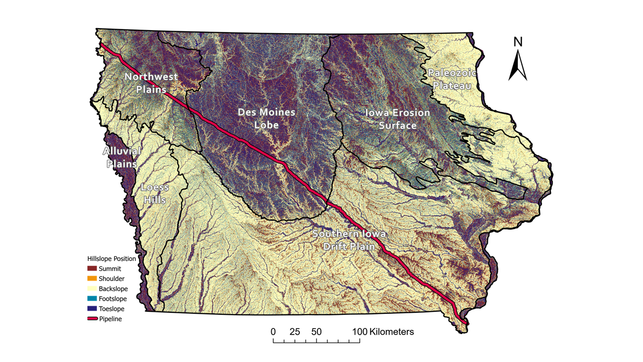
The hypothesis of this project is that soil health indicators capacity to recover their original condition after six years pipeline was installed will vary by parent material, landscape position, and management practices. Based on this, we defined the goal of creating a unique dataset of soil health indicators that covers the requirements to test our hypothesis. For this, two Iowa Physiographic Macro-Regions with distinctive characteristics were selected (Des Moines Lobe, and Southern Iowa Drift Plain). A questionnaire was designed to send to farmers affected by the installation of DAPL (Dakota Access Pipeline) in these two regions. To see the questionnaire access through the following link: https://iastate.qualtrics.com/jfe/form/SV_2rynEiRkmY6C8Mm
However, the efforts of trying to get farmers involved using the questionnaire were not successful. For this reason, an alternative method was applied. Farmers were contacted via phone to arrange a meeting with them on their farm where we explained the project, and we filled the questionnaire together with them. This process was more successful and done individually with each of the 14 farmers involved in the projects in the Des Moines Lobe and Southern Iowa Drift Plain (Figure 1).
The first round of interviews was completed in fall 2021 for farmers in the Des Moines Lobe, and the second round was completed in fall 2022 in the Southern Iowa Drift Plain. After each round of interviews was completed, we georeferenced each of the fields involved in the project. With the georeferenced data, we design the field samples collection along the DAPL path, stratifying locations by soil parent material, landscape position, management practices, and disturbed vs undisturbed areas. Once this information was set to each of the farms, sampling points were uploaded to the GPS before going to the field.
Besides the coordination with farmers, by law we also needed to coordinate with DAPL because we took samples over the pipeline. To complete this process, we needed to register to Iowa One Call and upload one ticket per field where we specify field location, sampling depth, purpose of the sampling, among other information. Once the tickets were approved, a representative person from DAPL contacted us and together with farmers we coordinated the visit to take samples on the different farms. The representative person of DAPL was present on each of the fields with a scanner that identifies the exact location of the pipeline, which helped us to be more precise by taking the samples from the exact place we planned.
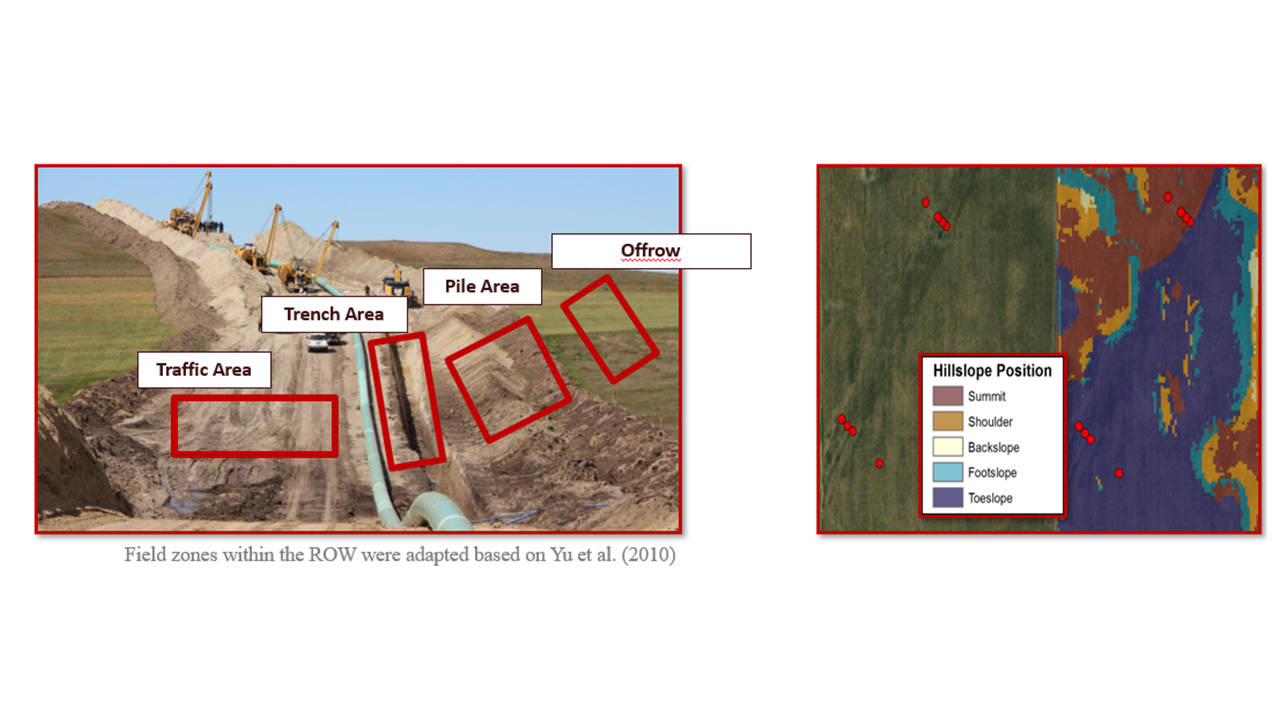
Once in the field, on each selected location, the pipeline path was divided into three parts: pile area, trench area, and traffic area which should represent each of the areas during the construction (Fig.2). Samples were collected for each of those points and on the undisturbed area every 30cm (about 12 in) to a depth of 90cm (about 3 ft) on the different hillslope positions presented on the different fields (Fig. 3). Each sample is duplicated because one was used for chemical, physical, and biological analysis, while the other was taken as a bulk density ring for hydrological measurements. Examples of soil cores with their respective bulk density rings and examples of soil cores of the different areas are represented in Figure 3.
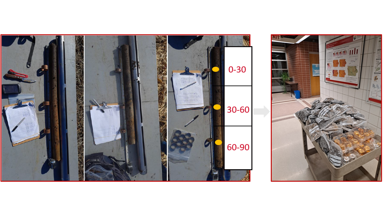
For the Des Moines Lobe, field sampling was finished in fall 2021. A total of 192 samples were taken which corresponds to 16 transects times 4 points per transect times 3 depths per point. After field sampling was completed, all samples were dried, grinded, and sieved to 2mm (about 0.08 in). For evaluation of microbial activity, CO2 burst test (Haney et al., 2008) was completed in November 2022. Soil particle size distribution was completed in December 2022 using a laser diffractometer (Miller & Schaetzl, 2012) for particle sizes’ role in hydrologic characteristics and as an indicator of soil mixing. For hydrologic properties, one ring of 3 cm height was taken every 30 cm (Figure 3) to construct the soil water retention curves until a matric potential of -15.0 bars, using a combination of ceramic plates and pressure chambers. In this case, the pressures used for measuring and build the water retention curves were: -0.10, -0.33, -1.0, -3.0, and -15.0 bars. On each run, we measured 36 rings at the same time, using a double ceramic plate per chamber. With this methodology we assessed porosity and relate the release of soil water under different suctions or matric potentials. Plant available water was calculated as the difference between volumetric water content at field capacity (-0.10 bars) and permanent wilting point (-15.0 bars). On the other hand, bulk density was calculated once each run was completed. To do this, rings were oven dried at 105 Celsius degrees until constant weight. After this, bulk density was calculated using the following formula: (solid mass (gr) / total volume of soil (cm3), and total porosity was calculated as follows: [1 - (Bulk density / Real density)] * 100], assuming a real density of 2.65 g/cm3.
For the Southern Iowa Drift Plain, field sampling was finished in fall 2022. A total of 276 samples were taken, which corresponds to 23 transects times 4 points per transect times 3 depths per point. As explained for the Des Moines Lobe, each sample also had a bulk density ring for hydrological measurements. After field sampling was completed, all samples were dried and sieved for chemical and physical analysis, while bulk density rings were used for hydrological measurements as described above.
To see report with pictures, see attached document: SARE_first_report
Field sampling and lab analysis for the Des Moines Lobe, and Southern Iowa Drift Plain regions was completed. All results from lab analysis are stored in our lab server. However, due to time constrains stemming from my graduation and subsequent return to my home country, I was only able to finalize the data analysis for central Iowa, leaving the analysis for southeast Iowa pending. Nevertheless, the intention is to fully complete the data analysis and subsequently publish the results in a peer-reviewed journal, which will be then uploaded as an information product of the current project.
- Results and discussions
3.1. Central Iowa
3.1.1 Field observations
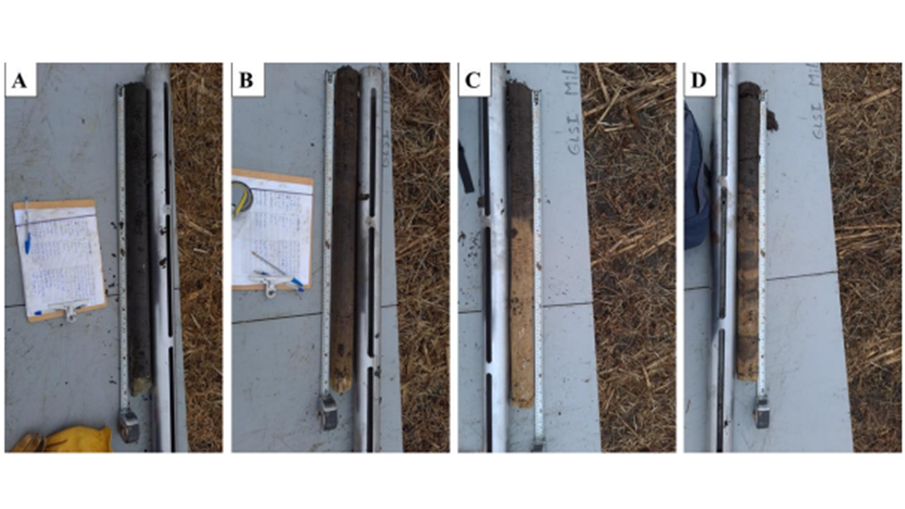
During the sampling campaign, notable visual differences were observed between the undisturbed area and the ROW. Among the ROW positions, the pile area exhibited the closest similarity to the undisturbed soil, while the traffic and trench areas displayed evident soil disturbance. Specifically, the traffic area was characterized by a reduction in the thickness of the A horizon, followed by a sudden transition to material from the C horizon, which often went unnoticed in the undisturbed area. On the other hand, the trench area exhibited a more consistent pattern, clearly indicating the mixing of topsoil with subsoil. This was evident from the lighter colors observed near the surface, representing the blending of the C horizon into the A and B horizons zone (Figure 4). Although this general trend was observed, it is important to note that variations were also observed among fields and within different ROW areas. These variations could be attributed to factors such as the specific pipeline installation crews and the field conditions during installation. However, it is worth mentioning that the trench area consistently exhibited clear evidence of subsoil mixing with the topsoil, regardless of the field location, parent material, or DHP.
trench
3.1.2. Physical properties
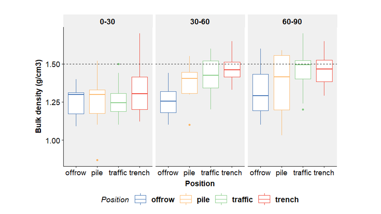
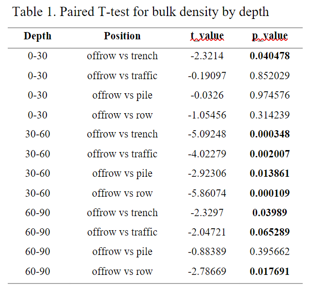
The trend in bulk density at various depths reveals elevated values across different positions within the ROW, particularly at depths ranging from 30-60 cm and 60-90 cm. Notably, the traffic and trench positions exhibit the highest bulk density values (Fig. 5). Statistical analysis detected significant differences between the undisturbed and trench positions within the 0-30 cm depth range, as well as across all positions within the ROW at depths of 30-60 cm and 60-90 cm, except for the pile position in the latter case (Table 1). These findings align with previous studies conducted by Naeth and Bailey (1987), Olson and Doherty (2012), Antille et al. 2016), and Tekeste et al. (2019), which reported elevated bulk density along pipeline ROWs. However, it's worth noting that while Naeth and Bailey (1987) found that this effect diminished below a depth of 60 cm, Antille et al. (2016) observed a 15% increase in bulk density in the top 30 cm of the ROW, which decreased to 5% between 30 cm and 70 cm. In contrast, in this study, the most significant differences in bulk density values between the undisturbed soil and the ROW occurred at depths of 30-60 cm and 60-90 cm, as illustrated in Figure 5.
When the bulk density results were examined by categories of DHP, a consistent trend emerged: higher bulk density values were consistently observed in the ROW areas in comparison to the undisturbed area, aligning with our previous observations. Notably, this trend was more pronounced on the toeslope than on the summit, with a notably higher frequency of values exceeding 1.5 g/cm³, especially at the 30-60 cm depth range (Fig. 6).
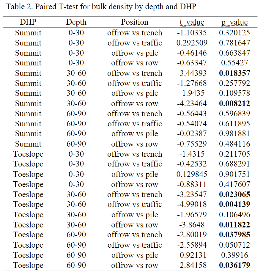
The statistical analysis revealed significant differences within the summit region at a depth of 30-60 cm, particularly within the trench area, as well as when comparing the undisturbed area to the ROW. On the toeslope, significant differences were observed between the undisturbed area and both the traffic and trench areas within the 30-60 cm depth range. Additionally, significant differences were observed from 60-90 cm between the undisturbed area and the trench, as well as between the undisturbed area and the ROW (Table 2).
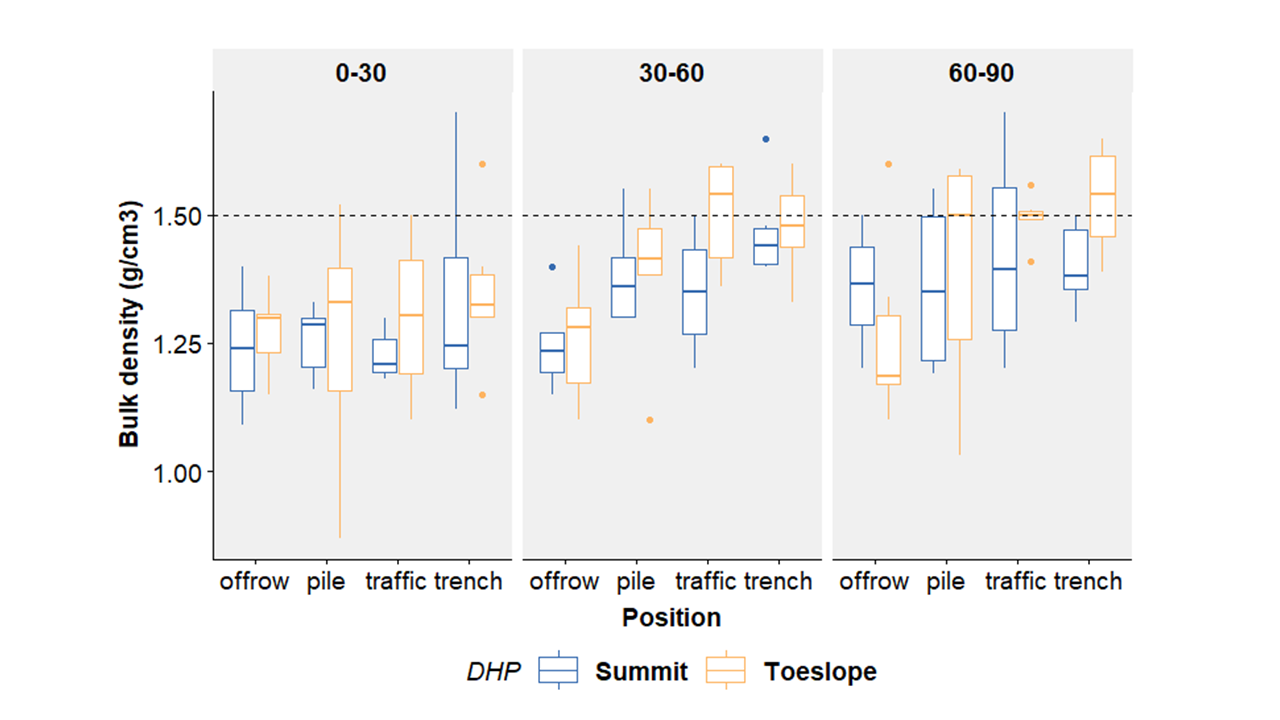
Figure 6. Bulk density by depth and DHP for the offrow and different ROW areas
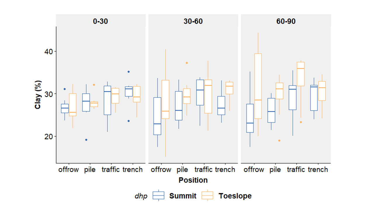
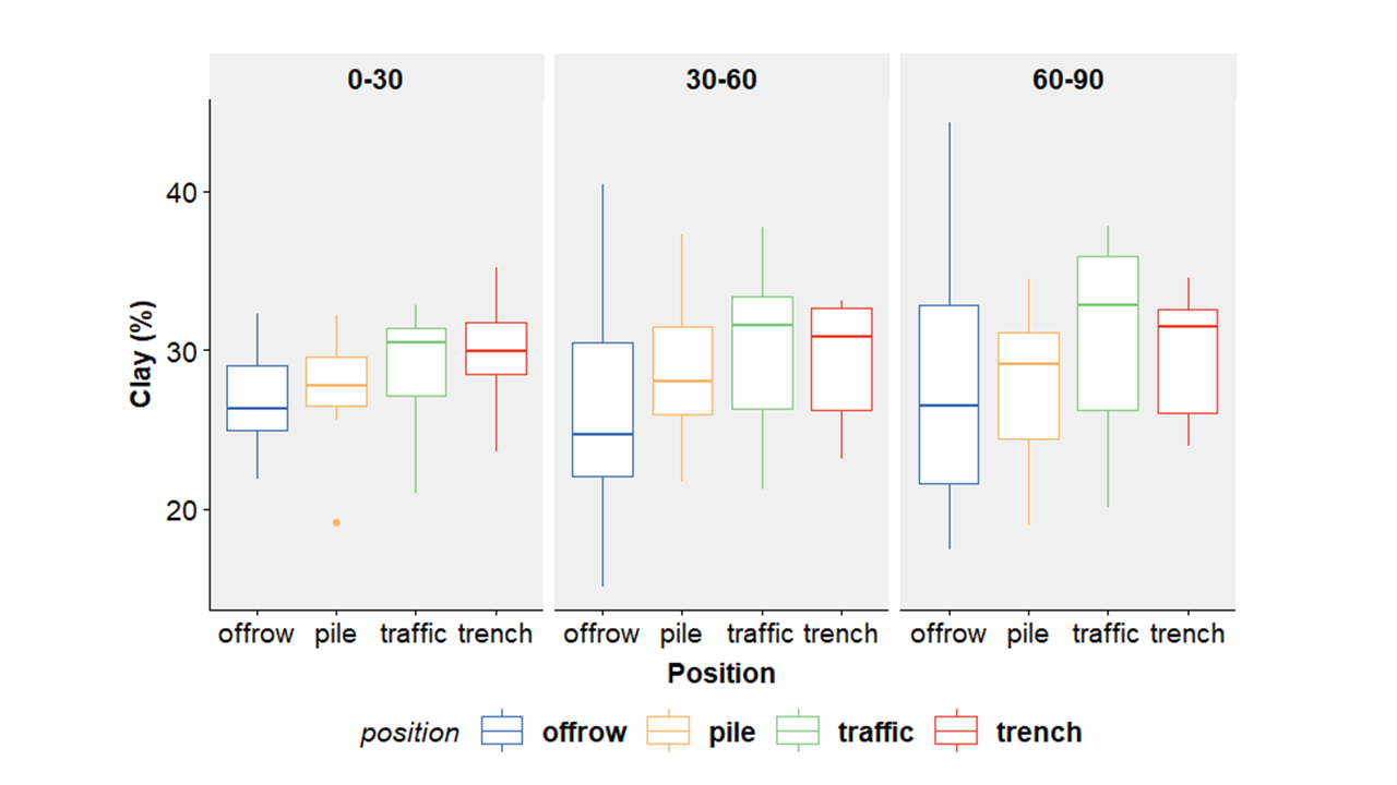
The soil's moisture content during installation plays a crucial role in soil compaction significantly influencing bulk density outcomes (Soane et al., 1980). Studies have shown that low soil moisture levels during installation can limit the increase in bulk density within the ROW (Nielsen, D., MacKenzie, A. F., Stewart, 1990). Consequently, the observed trend of elevated bulk density values on the toeslopes compared to the summits can be attributed to the moisture content present during the application of stress. This phenomenon can be explained by the addition of water, which acts as a lubricant between soil particles. This increased lubrication leads to enhanced cohesion and a more compact arrangement of soil particles. However, as the water content continues to rise, it begins to displace the soil particles. This is why, after reaching the maximum dry density, it starts to decrease. (Fig 7). Considering the toeslopes’ position in the landscape, together with the presence of higher clay content (Fig. 8), and shallow water tables, it is reasonable to expect more favorable moisture conditions during installation. This finding aligns with the research conducted by Olson and Doherty (2012) who reported extreme soil compaction values in wetland areas in Wisconsin.
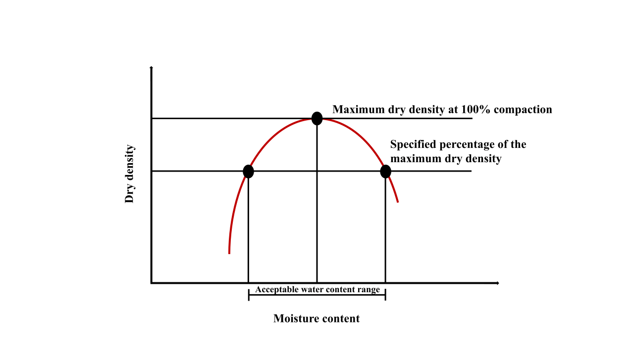
from Duncan, 1992)
Regarding the duration of compaction after pipeline installation, Shi et al. (2014) previously suggested that six years would be enough for the soil to recover. However, our findings contradict these results and align more closely with the observations made by Culley and Dow (1988) and (Olson & Doherty, 2012). Both studies reported higher bulk density values in the ROW even ten and eight years after installation, respectively. These results reinforce the viewpoint put forth by Hakansson and Reeder (1994), who reported that subsoil compaction appears to be nearly permanent. This perspective is further sustained by the study of Alakukku (1996) documented persistent subsoil compaction nine years after traffic-related activities. Additionally, Johansen et al. (2014) found that once the subsoil is compacted, the macropores reduction due to damage caused by compaction can endure for more than a decade.
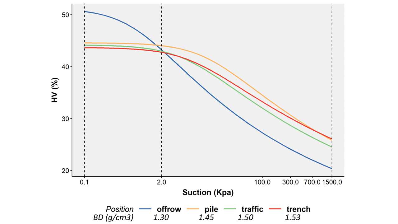
The influence of soil compaction on water retention exhibited depth-dependent variations, as depicted in Figures 9 and 10. Where statistical significance in bulk density differences was evident between offrow and ROW areas (Figure 9 in the trench area and Figure 10 in the pile, traffic, and trench areas), it became apparent that, near saturation, the volumetric water content was significantly higher in the offrow compared to the trench area at depths from 0-30 cm. A similar trend was observed when comparing offrow with all the ROW positions at depths from 60-90 cm. Conversely, beyond matric potential levels of 25 Kpa at depths from 0-30 cm and around 2 Kpa at depths from 60-90 cm, increasing compaction led to an increase in volumetric water content.
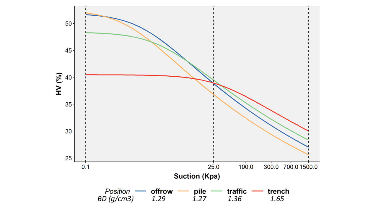
value
This phenomenon is noticeable in the trench position at depths from 0-30 cm and across all ROW positions at depths from 60-90 cm, resulting in a "flattening" of the water retention curves where significantly higher bulk density prevailed. This outcome can be attributed to the compaction-induced reduction of macropores, which, under the stress conditions, transform into mesopores and micropores, as observed by Hill and Sumner in 1967. In contrast, at 1500 Kpa, the opposite trend was evident. At this level of matric potential, a conspicuous reduction in volumetric water content is observed in offrow compared to trench conditions at depths from 0- 30 cm and between offrow and the various ROW positions at depths from 60-90 cm.
The "flattening" of the curves in more compacted soils can also be attributed to a reduction in total porosity and modifications in pore size distribution, as discussed by Smith and colleagues in 2001. This occurs because macropores are less resistant and weaker than micropores, causing them to shrink into smaller pores when subjected to stress.
This transformation of macropores into mesopores and micropores leads to decreased porosity during the compaction process. The visual representation of this transformation is apparent in the shift towards lower matric potentials in the S-curve shoulder as compaction intensifies (Figure 10), a phenomenon previously described by Smith et al. in 2001. Notably, at 1500 Kpa, the majority of water is localized within micropores. The reason
for the higher volumetric water content in compacted soil compared to less compacted soil lies in the higher bulk density of the former. Increased bulk density results in greater mass per unit of volume, consequently leading to a higher proportion of micropores and an increased specific surface area, defined as mass per unit of area (Horton, R. personal communication).
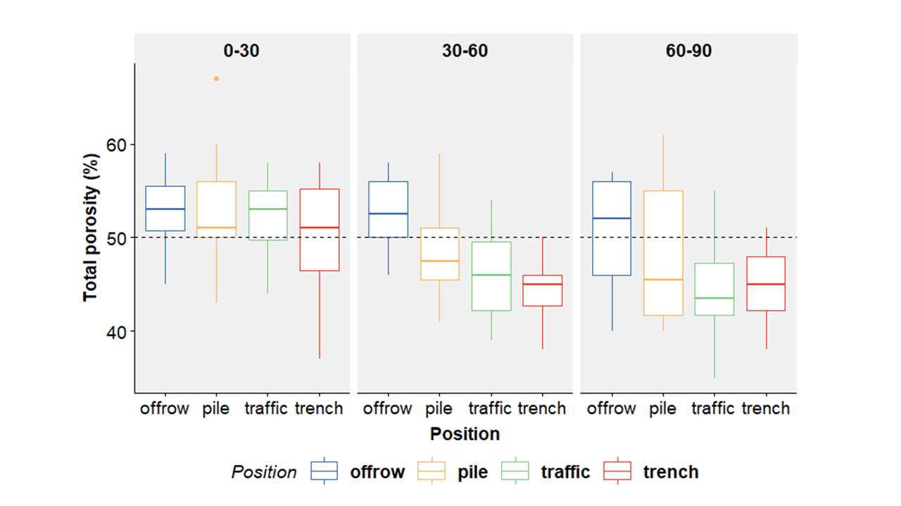
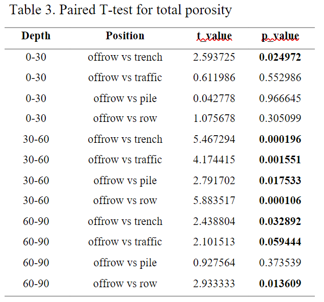
This effect is also notable when analyzing total porosity (Fig. 11). In the undisturbed position, total porosity maintains relatively consistent mean values across different depths. Conversely, significant reductions in total porosity are observed in the traffic and trench positions along the ROW. Statistical analysis underscores these differences in total porosity, particularly within the 0-30 cm depth range for the trench position and for the 60-90cm depths in most cases, as illustrated in Table 3. While the critical bulk density range for optimal corn root growth is reported to vary between 1.5 to 1.8 g/cm3
according to studies such as Bertrand and Kohnke (1957), Aune and Lal (1997), and the United States Department of Agriculture (USDA) (1999), it is noteworthy that yield reductions in corn following pipeline installation have been observed in the range of 15% to 43% when bulk density values reach 1.5 g/cm3 (Neilsen et al., 1990; Tekeste et al., 2020).
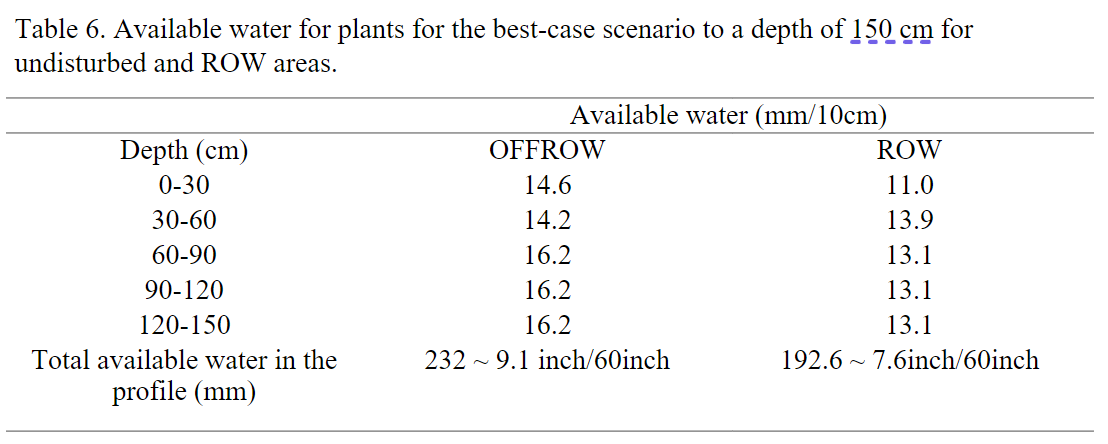
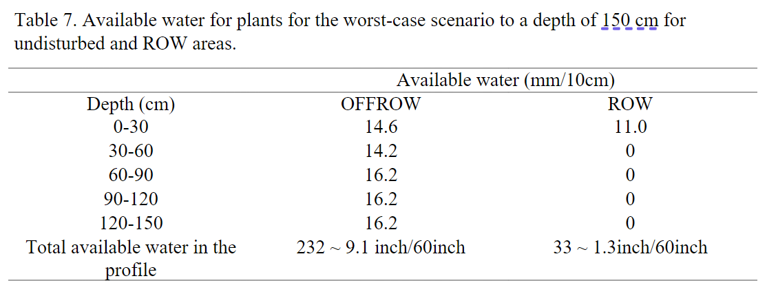
In the current study, our findings reveal that within the ROW, bulk density values exceeding 1.5 g/cm3 were consistently identified in the trench position across all depths. Additionally, in the traffic position, values exceeding 1.5 g/cm3 were observed at depths ranging from 30-60 cm and 60-90 cm. The study involved the calculation of available water for plant growth based on the average results obtained from both the undisturbed area and various ROW sections, as presented in Tables 4 and 5. Two distinct scenarios were taken into consideration: the best-case scenario, assuming that plant roots within the ROW could explore the entire profile, and the worst-case scenario, where roots in the ROW could only access the uppermost 30 cm of soil due to bulk density values exceeding 1.5 g/cm3 beyond this depth.
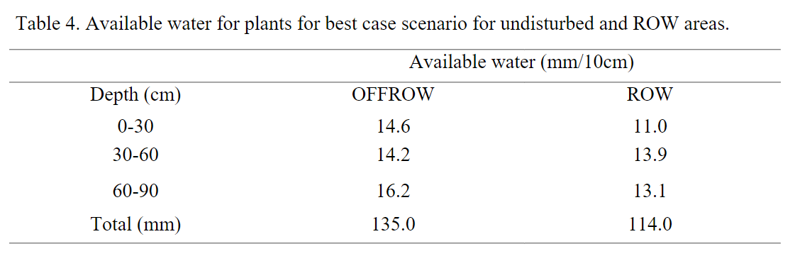
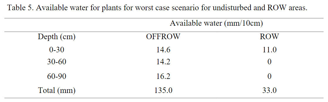
In both scenarios, it was evident that the undisturbed area consistently offered a higher volume of available water for plant growth in comparison to the ROW. Considering an estimated water usage of 5.6 mm/day for achieving an average corn yield of 13.5 tons/hectare in central Iowa (source: crops.extension.iastate.edu). It becomes apparent that the undisturbed area would sustain plant growth without additional rainfall for approximately 24 days. In contrast, the best-case scenario within the ROW would support growth for approximately 20 days, while the worst-case scenario would only provide six days of sustainable growth without rainfall.
CSR2 is an equation used in Iowa to estimate how suitable a soil is for producing corn using the maps and data from the Iowa Cooperative Soil Survey (ICSS). It is composed of six parameters and its range goes from 0 to 100, being 100 the perfect conditions for producing corn. CSR2 = S – M – W – F – D +/- EJ Where: S is the taxonomic subgroup class of the series of the soil map unit (MU), M is the family particle size class, W relates to the available water holding capacity of the series, F is the field condition of a particular MU (slope, flooding, ponding, erosion class and topsoil thickness), D is the soil depth and tolerable rate of soil erosion, and EJ is an expert judgment correction factor (Burras, Miller, Fenton, and Sassman, 2015). Considering this, CSR2 was estimated based on the two proposed scenarios of available water for plants. Since CSR2 estimations rely on a 150 cm profile, results from 60-90 cm were extrapolated to 90-120 cm and 120-150 cm to ensure compatibility in the calculations (Tables 6 and 7).
For the Clarion soil series found in central Iowa that belongs to the Typic Hapludolls taxonomic subgroup, an S factor 100. The M factor was determined as four based on its fine-loamy particle size class. The W factor was assigned a value of 0 for the undisturbed area and 8 for the ROW. No restrictions were identified for slope, flooding, ponding, erosion class, topsoil thickness, and tolerable rate of erosion, resulting in F factor, D factor, and EJ factor all being 0. Additionally, the equation 1.6 * CSR2 + 80 was used to calculate the corn yield (Dr. Burras personal communication).
CSR2 NO RESTRICTIONS = 100-0-0-0-0-0 = 100 ~ 1.6 * 100 + 80 = 240 bu/acre
CSR2 OFFROW = 100-4-0-0-0-0 = 96 ~ 1.6 * 96 + 80 = 233.6 bu/acre (6.5% yield loss)
CSR2 ROW = 100-4-8-0-0-0 = 88 ~ 1.6 * 88 + 80 = 220.0 bu/acre (12% yield loss)
For the worst-case scenario, all factors remain the same except for the W factor, which would change to 24 based on the calculations using the available water values from Table 7. This adjustment is made because the available water is less than 3 inches/60 inches. Based on this information:
CSR2 ROW = 100-4-24-0-0-0 = 72 ~ 1.6 * 72 + 80 = 195.2 bu/acre (22% yield loss)
These yield reductions estimated above are similar to the ones found by Ebrahimi et al. (2022), which uses APSIM to measure corn and soybean growth and water use on a disturbed field by the same pipeline in Iowa. These authors found yield reductions for soybean and corn being 20% and 27%, respectively.
3.1.2. Chemical properties
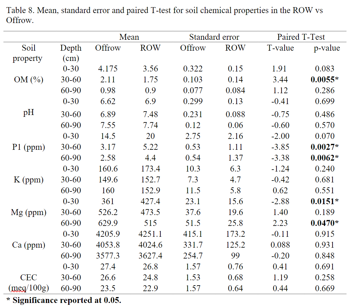
In general, for chemical properties, statistically significant differences were observed for OM at 30-60 cm, P1 from 40-60 cm and 60-90 cm, Mg 0-30 cm and 60-90 cm (Table 8). However, in comparison with physical properties, the effects caused by DAPL installation are less noticeable.
Soil pH is one of the most important soil properties due to its pivotal role in regulating the availability of essential nutrients for plants (Robson, 1989). Plant growth can be constrained by pH values exceeding eight due to the unavailability of essential nutrients, such as phosphorus (P), at such elevated levels (Jensen, 2010). The mixing of subsoil with topsoil, resulting in the incorporation of carbonaceous material from the subsoil, leads to substantial increases in topsoil pH. These pH increases are typically accompanied by an elevation in CaCO3 content. This combination of factors, including the introduction of alkaline materials and the dilution of soil organic matter (SOM), contributes to the overall rise in soil pH within the ROW (Birkhimer et
al., 2023). As a result, the buffer capacity of the topsoil pH is diminished.
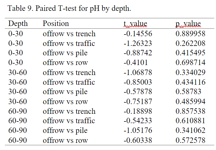
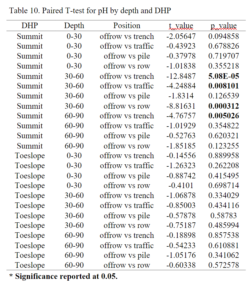
For pH, results from this study coincide with previous results (Harper &Kershaw, 1997; Ivey & McBride, 1999; Kowaljow & Rostagno, 2008; Shi et al., 2015; Zellmer et al., 1985) where no significant change in pH was observed in the ROW versus undisturbed area. However, in the present study, a trend of increasing pH on the ROW was noticed (Fig. 12). When data was analyzed by DHP (Fig. 13), distinct differences in pH values between the summit and toeslope became apparent, particularly for the 0-30 cm and 30-60 cm depths. In this case, statistically significant differences were observed in the summit region at 30-60 cm for the trench, traffic, and ROW areas compared to the undisturbed area. Additionally, significant differences were found between the undisturbed area and the trench area from 60-90 cm depth (Table 9).
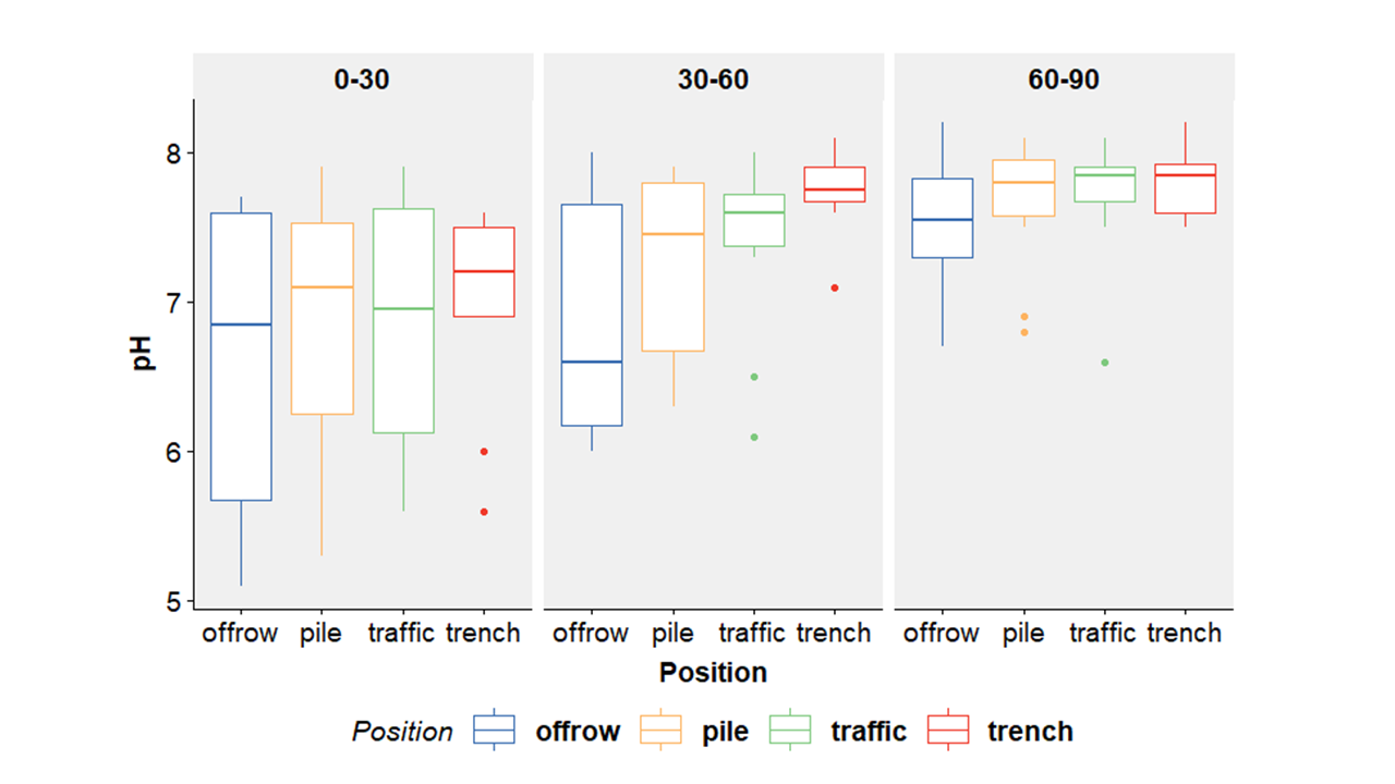
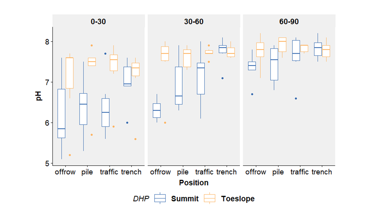
These findings highlight the influence of DHP on pH variations within the ROW, emphasizing the distinct pH dynamics between the summit and toeslope sections. In central Iowa, this is expected because salts like calcium carbonate have the ability to be washed out from the higher elevations of the hillslope and transported towards the lower regions through the movement of groundwater. Subsequently, they are drawn back up in the soil profile through capillary suction when the surface soil dries out due to evaporation processes. This process is responsible for observing higher pH in the toeslope compared to the summit (Ritcher and Burras, 2017).
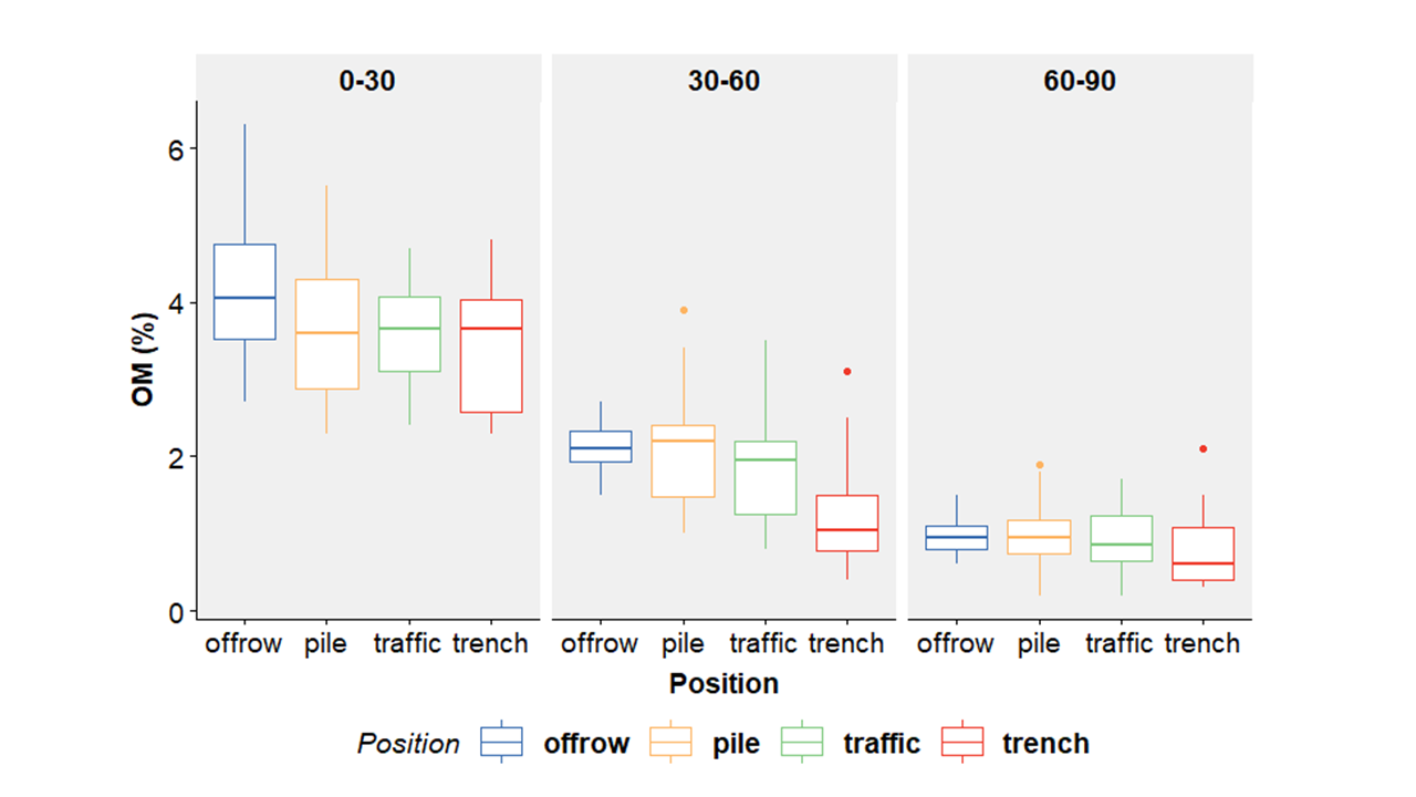
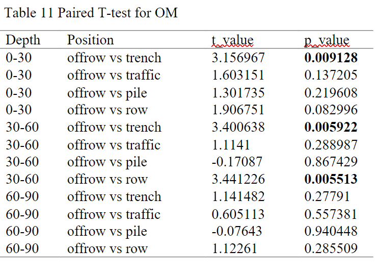
SOM results showed an inverse relationship with soil pH. The inverse relationship between pH and SOM can be explained because SOM has a high CEC and the ability to hold H+ ions in the soil (Ji et al., 2014). For this property, there is a trend of lower OM values in the different ROW positions versus the undisturbed area (Fig. 14). However, significant differences were identified only from 0-30 and 30 to 60 cm on the trench area (Table 11). This observed trend agrees with the results found by Naeth and Bailey (1987), Soon et al. 2000; and Shi et al., 2014, who reported reductions in SOC due to the mixing of subsoil with surface layers. According to Birkhimer et at. (2023), labile SOM losses due to pipeline installation procedures cannot be avoided because when soil is removed, stocked in a pile, and later respread in the site promotes an increment in C mineralization (Mason et al., 2011) and notable temporary rises in microbial biomass (Soon, Rice et al., 2000).
In the case of P1, statistically significant differences were found between the undisturbed and ROW, but in this case, higher P1 values were found on the ROW (Table 8). In previous works, generally no significant differences were found between the undisturbed and ROW areas. However, studies that found differences (Soon, Rice et al. 2000) observed lower pH values after the first year of reclamation, and attributed decreases on P in the ROW due to the pH increment due to the mixing of subsoil with topsoil. The findings from our study do not align with these results, as increases in both pH and P1 in the ROW were observed. Possible explanations for this discrepancy could be the implementation of farming practices aimed at improving growth conditions in the ROW, which may have resulted in higher P application rates that are reflected in the soil analysis.
Regarding Mg, also there is a lack of information about possible changes due to the non-observation of pipeline installations effects on this nutrient (Birkhimer et al. (2023). However, Wester et al. (2019) observed a decrease in Mg levels after pipeline installation probably because of nutrient loss through percolation across several consecutive growing periods. In our case, results vary depending on the depth. From 0-30 cm significant differences were observed but in favor of ROW, because Mg values are higher in these areas compared to the undisturbed area. In contrast at 60-90 cm depth although significant differences were also observed, in this case the undisturbed area is the one with higher Mg values compared to the ROW (Table 8).
For particle size distribution, although a trend of higher clay content on the different ROW areas was found in comparison with the undisturbed area, in general, and when the analysis was performed by DHP (Fig. 15 and 8 respectively), no statistically significant differences were observed for CEC,
which has been reported by Culley and Dow (1988); Culley and Dow (1982) that an increase in clay content is accompanied by an increase in CEC.
References
Alakukku, L. (1996). Persistence of soil compaction due to high axle load traffic. I. Short-term effects on the properties of clay and organic soils. Soil and Tillage Research, 37(4), 211-222.
Antille, D. L., Huth, N. I., Eberhard, J., Marinoni, O., Cocks, B., Poulton, P. L., Macdonald, B. C. T., & Schmidt, E. J. 2016. The effects of coal seam gas infrastructure development on arable land in Southern Queensland, Australia: Field investigations and modeling. Transactions of the ASABE, 59(4), 879–901. https://doi.org/10.13031/trans.59.11547
Aune, J. B., & Lal, R. (1997). Agricultural productivity in the tropics and critical limits of properties of Oxisols, Ultisols, and Alfisols. Tropical Agriculture.
Bertrand, A. R., & Kohnke, H. (1957). Subsoil conditions and their effects on oxygen supply and the growth of corn roots. Soil Science Society of America Journal, 21(2), 135-140.
Birkhimer, N., DeSutter, T. M., Jore, K., Staricka, J., & Meehan, M. (2023). Effects of pipeline and well‐pad reclamation on topsoil properties: A meta‐analysis. Agrosystems, Geosciences & Environment, 6(2), e20387.
Burras, C. L., Miller, G. A., Fenton, T. E., & Sassman, A. M. (2015). Corn suitability rating 2 (CSR2) equation and component values. Connolly, R., Freebairn, D., Bell, M., & Thomas, G. (2001). Effects of rundown in soil hydraulic condition on crop productivity in south- eastern Queensland: A simulation study. Australian Journal of Soil Research, 39(5), 1111–1129. https://doi.org/10.1071/SR00089
Culley, J. L. B., & Dow, B. K. (1988). Long-term effects of an oil pipeline installation on soil productivity. Canadian journal of soil science, 68(1), 177-181.
Culley, J. L., Dow, B. K., Presant, E. W., MacLEAN, A. J., & MecLsAN A J, E. W. 1982. Recovery of productivity of Ontario soils disturbed by an oil pipeline installation. Canadian Journal of Soil Sciences, 62, 267-279.
De Jong, E., & Button, R. C. 1973. Effects of pipeline installation on soil properties and productivity. Canadian Journal of Soil Science 53, 37-47. https://doi.org/10.4141/cjss73-005
Ebrahimi, E., Tekeste, M. Z., Huth, N. I., Antille, D. L., Archontoulis, S. V., & Horton, R. (2022). Measured and modeled maize and soybean growth and water use on pipeline disturbed land. Soil and Tillage Research, 220, 105340.
Haney, R. L., Brinton, W. F., and Evans, E. 2008. Soil CO2 respiration: Comparison of chemical titration, CO2 IRGA analysis, and the Solvita gel system. Renew. Agric. Food Syst. 23, 171– 176. https://doi.org/10.1017/S174217050800224X
Håkansson, I., & Reeder, R. C. (1994). Subsoil compaction by vehicles with high axle load extent, persistence and crop response. Soil & Tillage Research, 29, 277-304. https://doi.org/10.1016/0167-1987(94)90065-5
Harper, K. A., & Kershaw, G. P. (1997). Soil characteristics of 48-year-old borrow pits and vehicle tracks in shrub tundra along the CANOL No. 1 pipeline corridor, Northwest Territories, Canada. Arctic and Alpine Research, 29(1), 105-111.
Hill, J. N. S., & Sumner, M. E. (1967). Effect of bulk density on moisture characteristics of soils. Soil Science, 103(4), 234-238.
Horton, R., Ankeny, M.D., Allmaras, R.R., 1994. Effects of compaction on soil hydraulic properties. Dev. Agric. Eng. 11, 141–165. https://doi.org/10.1016/b978
Iowa State University, Crops extension. (2023). https://crops.extension.iastate.edu
Ivey, J. L., & McBride, R. A. (1999). Delineating the zone of topsoil disturbance around buried utilities on agricultural land. Land Degradation & Development, 10(6), 531-544.
Jensen, T. (2010). Soil pH and the availability of plant nutrients. International Plant Nutrition Institute, Plant Nutrition Today.
Ji, C.-J., Yang, Y.-H., Han, W.-X., He, Y.-F., & Smith, J. (2014). Cli- matic and edaphic controls on soil pH in alpine grasslands on the Tibetan Plateau, China: A Quantitative analysis. Pedosphere, 24, 39–44.
Johansen, T. J., Thomsen, M. G., Løes, A. K., & Riley, H. 2015. Root development in potato and carrot crops – influences of soil compaction. In Acta Agriculturae Scandinavica Section B: Soil and Plant Science, 65 (2), 182–192. Taylor and Francis Ltd. https://doi.org/10.1080/09064710.2014.977942
Kowaljow, E., & Rostagno, C. M. (2008). Gas-pipeline installation effects on superficial soil properties and vegetation cover in Northeastern Chubut.
Mason, A., Driessen, C., & Norton, J. (2011). First year soil impacts of well-pad development and reclamation on Wyoming’s Sagebrush Steppe. Natural Resources and Environmental Issues, 17,5.
McConkey,
Miller, B. A., & Schaetzl, R. J. (2012). Precision of soil particle size analysis using laser diffractometry. Soil Science Society of America Journal, 76(5), 1719-1727.
Naeth, & Bailey. 1987. Persistence of changes in selected soil chemical and physical properties after pipeline installation in solonetzic native rangeland. In Can. J. Soil. Sci. https://doi.org/10.4141/cjss87-073
Neilsen, D., MacKenzie, A. F., & Stewart, A. (1990). The effects of buried pipeline installation and fertilizer treatments on corn productivity on three eastern Canadian soils. Canadian journal of soil science, 70(2), 169-179.
Olson, E. R., & Doherty, J. M. 2012. The legacy of pipeline installation on the soil and vegetation of southeast Wisconsin wetlands. Ecological Engineering, 39, 53–62. https://doi.org/10.1016/j.ecoleng.2011.11.005
PHMSA. 2020. Annual Report Mileage Summary Statistics. U.S. Department of Transportation. https://www.phmsa.dot.gov/data-and-statistics/pipeline/annual-report-mileage-summary-statistics (accessed 14 June 2021)
Richter, J. L., & Burras, C. L. (2017). Human-Impacted Catenas in North-Central Iowa, United States: Ramifications for Soil Mapping. In Soil mapping and process modeling for sustainable land use management (pp. 335-363). Elsevier.
Robson, A. D. (1989). Soil acidity and plant growth. Academic Press.
Shi, P., Xiao, J., Wang, Y. F., & Chen, L. D. 2014. The effects of pipeline construction disturbance on soil properties and restoration cycle. Environmental Monitoring and Assessment, 186(3), 1825–1835. https://doi.org/10.1007/s10661-013-3496-5
Smith, C., Johnston, M., & Lorentz, S. (2001). The effect of soil com- paction on the water retention characteristics of soils in forest plan- tations. South African Journal ofPlant and Soil, 18(3), 87–97. https: //doi.org/10.1080/02571862.2001.10634410
Soon, Y. K., Arshad, M. A., Rice, W. A., & Mills, P. 2000. Recovery of chemical and physical properties of boreal plain soils impacted by pipeline burial. Canadian Journal of Soil Science, 80, 489-497. https://doi.org/10.4141/S99-097
Tekeste, M. Z., Hanna, H. M., Neideigh, E. R., & Guillemette, A. 2019. Pipeline right-of-way construction activities impact on deep soil compaction. Soil Use and Management 35(2), 293–302. https://doi.org/10.1111/sum.12489
Wester, D., Hoffmann, J., Rideout-Hanzak, S., Ruppert, D., Acosta- Martinéz, V., Smith, F., & Stumberg, P. (2019). Restoration of mixed soils al pipelines in the western Rio Grande Plains, Texas, USA. Journal of Arid Environments, 161, 25–34. https://doi.org/10.1016/ j.jaridenv.2018.10.002
Zellmer, S. D., Taylor, J. D., & Carter, R. P. (1985, January). Edaphic and crop production changes resulting from pipeline installation in semiarid agricultural ecosystems. In national meeting of the American Society for Surface Mining and Reclamation. Denver, Colorado.
Educational & Outreach Activities
Participation summary:
In November 14th 2023 I conducted an online meeting where I presented for the interested farmers the results we had for central Iowa.
Project Outcomes
This study provides valuable insights into the long-term impacts of pipeline installation on agricultural sustainability. The findings highlight the significant effects on soil health indicators, particularly physical properties such as bulk density, total porosity, and available water for plants, six years post-installation. Notably, the reduction in available water for plants can lead to yield reductions of up to 12% in the best-case scenario and up to 22% in the worst-case scenario where bulk density values exceed 1.5g/cm3.
The project contributes crucial data to the existing body of knowledge, demonstrating soi degradation as associated economic losses persisting for more than six years post-installation. This evidence underscores the importance of adhering to installation protocols to mitigate adverse impacts on soil health and agricultural productivity.
This project allows farmers to gain access to objective information to evaluate the real impacts on land value and production, facilitating fair compensation determination. Moreover, knowing which soil health indicator has been more affected, allows them to switch from their current random treatments, and focus on practices that helps them on overcome that limitation. Ultimately, the findings emphasize the need for informed decision-making and policy interventions to address the challenges posed by soil degradation resulting from pipeline installation, thereby safeguarding agricultural sustainability for current and future generations.
Among the different dynamic soil properties studied, physical properties, especially bulk density, and consequently, total porosity and available water for plants were the most affected six years after pipeline installation. The reduction in available water for plants in the best-case scenario, produces a yield reduction of around 9%. However, in the worst-case scenario where bulk density values surpass values of 1.5 g/cm3 , yield reductions due to limitations in available water for plants can reach 20%. Overall, there were no statistically significant differences observed for the chemical properties. However, many of the trends were consistent with previous studies, where higher pH levels and lower organic matter content were observed as a result of the mixing of subsoil with topsoil.
From a farmer in Central Iowa: "This study adds important data to a growing body of information, which conclusively demonstrates that soil degradation and related economic losses are incurred for more than six years. Results of this work provide evidence that this damage to soil is occurring regardless of soil environment but is most drastic when protocols for installation were not followed. By making this data publicly available, stakeholders will have access to objective information for determining fair compensation for real impacts on land value and production. The extent of this soil degradation is also worth consideration in discussions about US food security, and the US as a provider for world food supply as well. Loss of soil productivity due to pipeline installation is one more factor decreasing the amount of prime farmland in the US, which is an issue for public policy at the state and federal levels".