Final report for GW18-024

GW18-024 (project overview)

Project Type: Graduate Student

Funds awarded in 2018: $25,000.00

Projected End Date: 04/30/2021

Grant Recipient: University of Arizona

Region: Western

State: Arizona

Graduate Student:

Scott Jones

Principal Investigator:

Steven Archer

The University of Arizona

Expand All Collapse All

Project Information

Summary:

Many rangelands have experienced shrub encroachment in concert with the loss of native grasses. Efforts to combat this phenomenon include a variety of ‘brush management’ practices (BM) traditionally aimed at restoring losses in forage production that occur when shrubs proliferate: but such practices are seldom economically viable from that standpoint. However, shrub encroachment also affects numerous other ecosystem services (ESs). A broader evaluation of the impacts of shrub encroachment and BM on ES would enable: (i) more accurate assessments of the utility of BM and (ii) development of guidelines for determining when, where and under what circumstances to use BM to promote a broader suite of desired ESs. Shrub encroachment/BM influences on ES are locally constrained by soils, topography, natural disturbance, and livestock grazing, but no conceptual framework integrating these factors with ES presently exists. This project aims to take a holistic approach to the shrub encroachment phenomenon, how it has altered ESs and the ability of BM to recover and restore valued lost services.

Outcomes will include:

(1) Improved understanding of producer demands for ESs on shrub-encroached landscapes

(2) Enhanced knowledge of shrub encroachment/BM patterns and processes

(3) Improved targeting of range management planning and practices by characterizing spatiotemporal changes in ES, and

(4) Assessments of ES trade-offs/synergies associated with shrub encroachment/BM in rangeland environments.

To achieve these outcomes, I have been (i) quantifying rates/patterns of shrub cover across the Las Cienegas National Conservation Area (LCNCA), a working rangeland, with contrasting soils, topography, and management histories in order to (ii) set baseline levels of ESs and (iii) identify maximum potential shrub cover based on topo-edaphic variables. This information is being used to (iv) model how future shrub encroachment/BM actions will impact capacities of stakeholder-desired ES. Recent and ongoing outreach activities have included presentations at local workshops, annual meetings of the Society for Range Management, and county-level Cooperative Extension programs. Written documents (e.g. fact sheets, articles for popular outlet and peer-reviewed scientific journals) are in draft stages at this writing.

Project Objectives:

The overarching goal of this project is to take a holistic approach to the shrub encroachment phenomenon, how it has altered ESs and the ability of brush management to restore services valued by stakeholders.

Specific objectives are to:

(1) Identify and rank producer demands for rangeland ESs through semi-structured interviews and surveys.

(2) Characterize spatial and temporal dynamics of shrub cover on sites with

a) contrasting soils and topography, and

b) known histories of brush management

(3) Model spatiotemporal ecosystem service capacity using

a) Land cover classifications from (2), and assign ES values based upon field data and peer-reviewed literature, and

b) Statistical analysis to evaluate relationships between multiple ESs and identify possible trade-offs and synergies.

Research

Materials and methods:

Objective 1: Identify and weigh producers’ demands for rangeland ES.

Objective 1: Identify and rank producer demands for rangeland ESs.

Pre-Test:

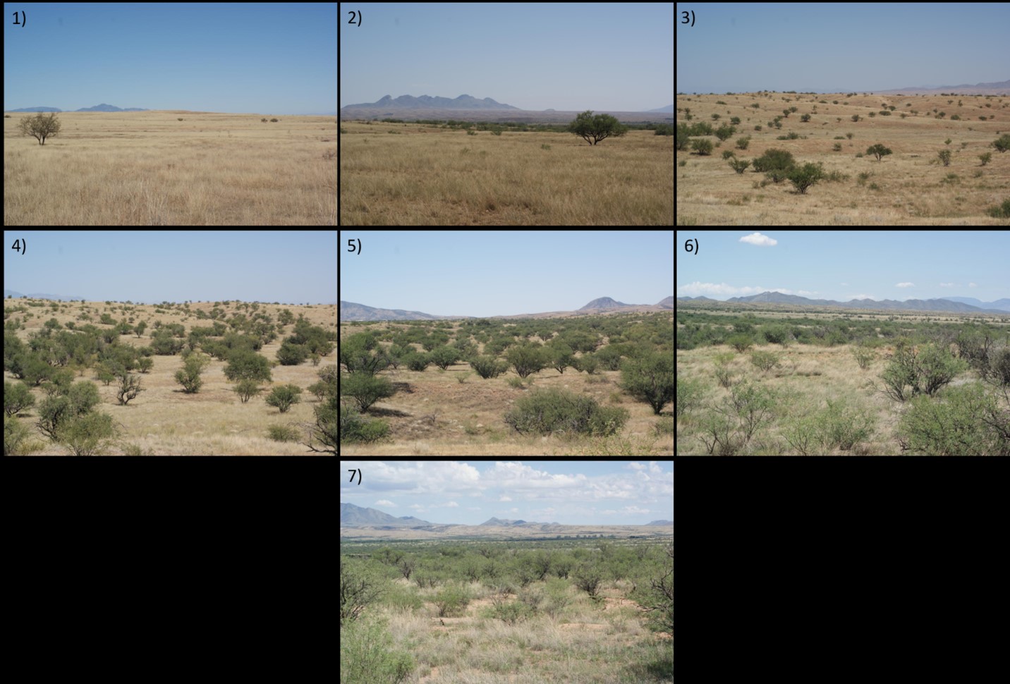
Semi-structured interviews were conducted between November 2019 and July 2020 with stakeholder groups that included producers, governmental employees, non-governmental land managers, and academicians. The interview contained closed- and open-ended questions concerning participants’ knowledge of issues relevant to this study. Focal topics included (i) shrub encroachment and its environmental impacts, and (ii) brush management and motives/rationale for deploying this management tool. An example of this semi-structured interview can be found here: https://projects.sare.org/wp-content/uploads/Appendix-1.png). Images of rangelands with differing shrub cover (Figure 1) were used to ascertain participants’ preferred degrees of shrub cover and the level of shrub cover at which they would consider implementing brush management. Participants were also asked to review and rank a list of 16 ecosystem services. A total of 18 participants were interviewed. Insights from this pre-test was used to create an online survey. Based on responses from the semi-structured interviews, images were updated, and the list of ecosystem services was pared down to focus on the 7 services deemed most important.

Figure 1. Photographs presented to participants during semi-structured interviews showing areas with differing shrub cover. 1) No shrubs; 2) Low cover; 3) Medium-low cover; 4) Medium cover; 5) Medium-high cover; 6) High cover; 7) Closed shrub canopy. Participants were asked to order images from most- to least-preferred based on their aesthetic appeal and by the ecosystem services provided. Participants are also asked to identify which image would represent the level of shrub cover at which brush management should be undertaken.

Online Survey:

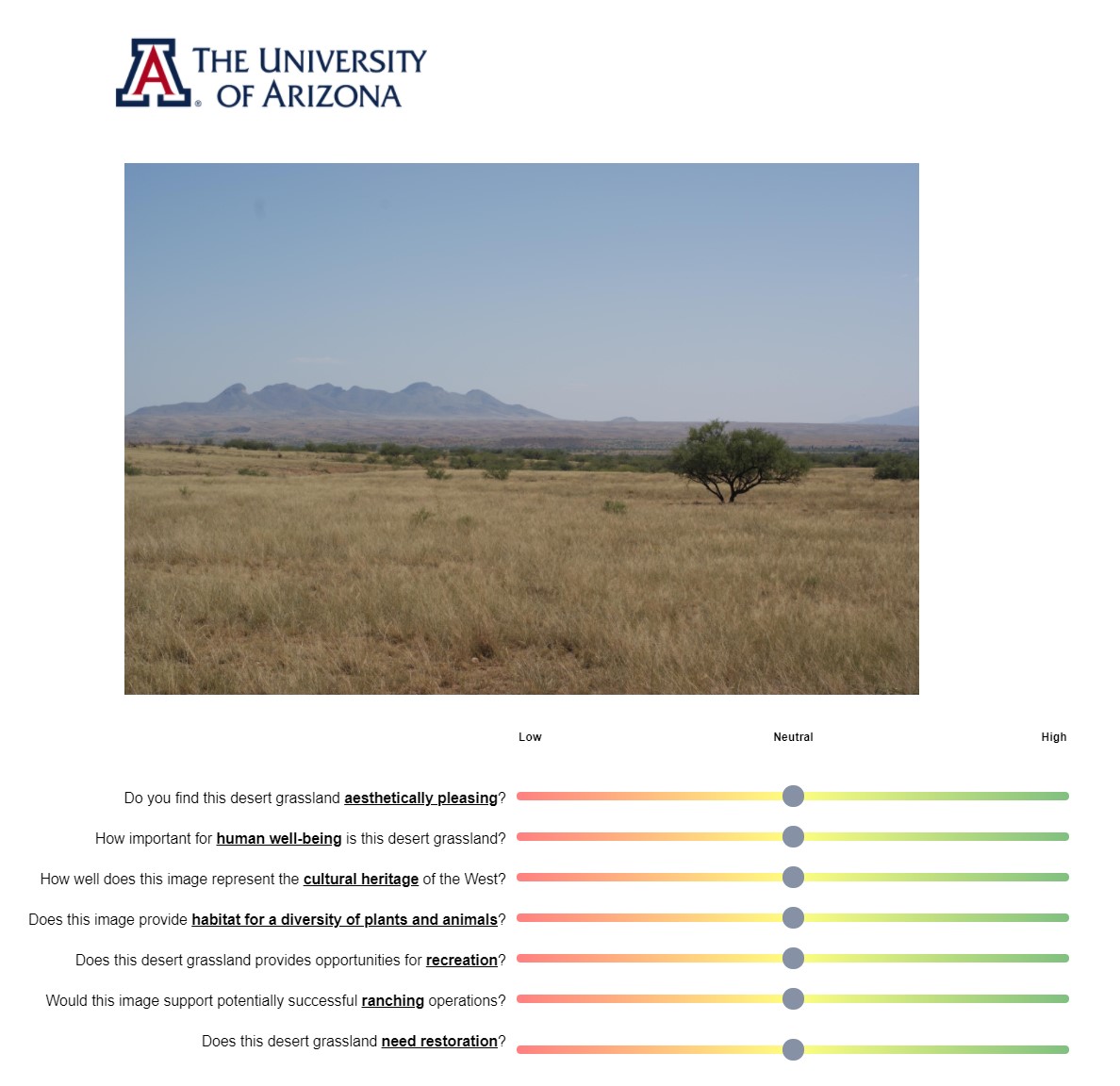
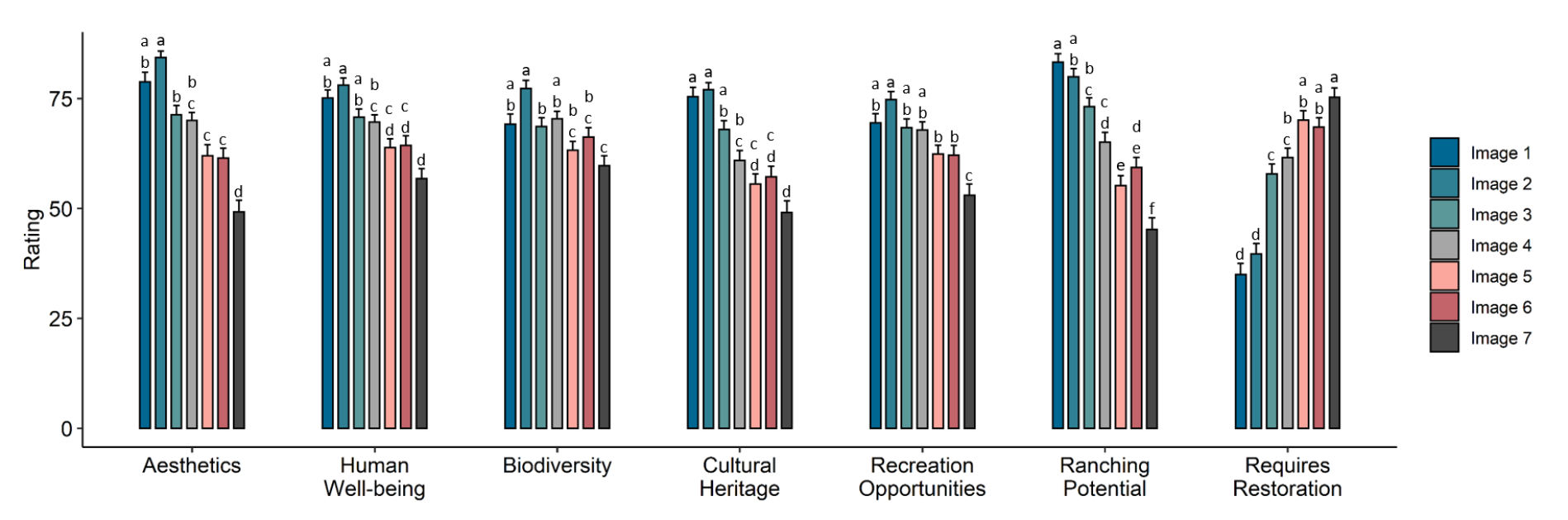
An online survey using the Qualtrics platform was distributed to stakeholders in Southern Arizona and New Mexico on November 29, 2020 with a follow-up distribution on February 8, 2021. Stakeholder groups targeted for the survey included producers, governmental employees, non-governmental land managers, academicians, and people who recreate and/or live near rangelands. The survey consisted of three sections. The first section consisted of an image-based survey. Participants were shown the photos in Figure 1 and asked to score the panels according to six characteristics with respect to: aesthetics, importance to human well-being, cultural heritage, habitat for biodiversity, recreation/ranching opportunities, and whether or not brush management should be undertaken (Figure 2). A Post-hoc Tukey pairwise comparison tested for differences for each variable across each image and Spearman’s rank correlation coefficients were computed from participant scores for the aforementioned characteristics to measure the strength of the associations between these quantitative variables.

In the second section, a Best Worst Scaling approach (Figure 3; Flynn et al. 2007) was used to rank participant perceptions of a suite of seven ecosystem services (water quality, biodiversity, erosion control, aesthetic value, cultural heritage, recreation/tourism and forage potential). A Balanced Incomplete Block Design (BIBD) was used, wherein each service was shown to participants four times and compared to each other service a total of two times. Conditional logit models were used to analyze the relative importance of each ecosystem service preference and a Wald p-Test was used to compare these services. The third and final section collected basic demographic information for survey respondents. The full online survey can be explored using the following link: https://uarizona.co1.qualtrics.com/jfe/form/SV_0OHbRHfRCXpcfFc

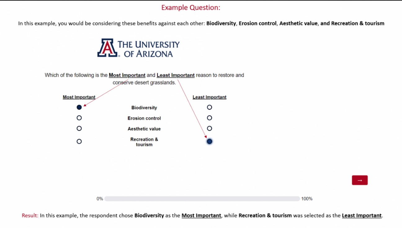
Figure 3. Example Best Worst scaling question from Section 2 of the online survey. Survey design used a balanced incomplete box to rate best and worst of seven ecosystem services (water quality, biodiversity, erosion control, aesthetic value, cultural heritage, recreation/tourism and forage potential). Each service was shown a total of four times and was rated against each other service twice

Objective 2: Characterize spatial and temporal dynamics of shrub cover on both shrub-encroached and managed sites with contrasting soils, topography.

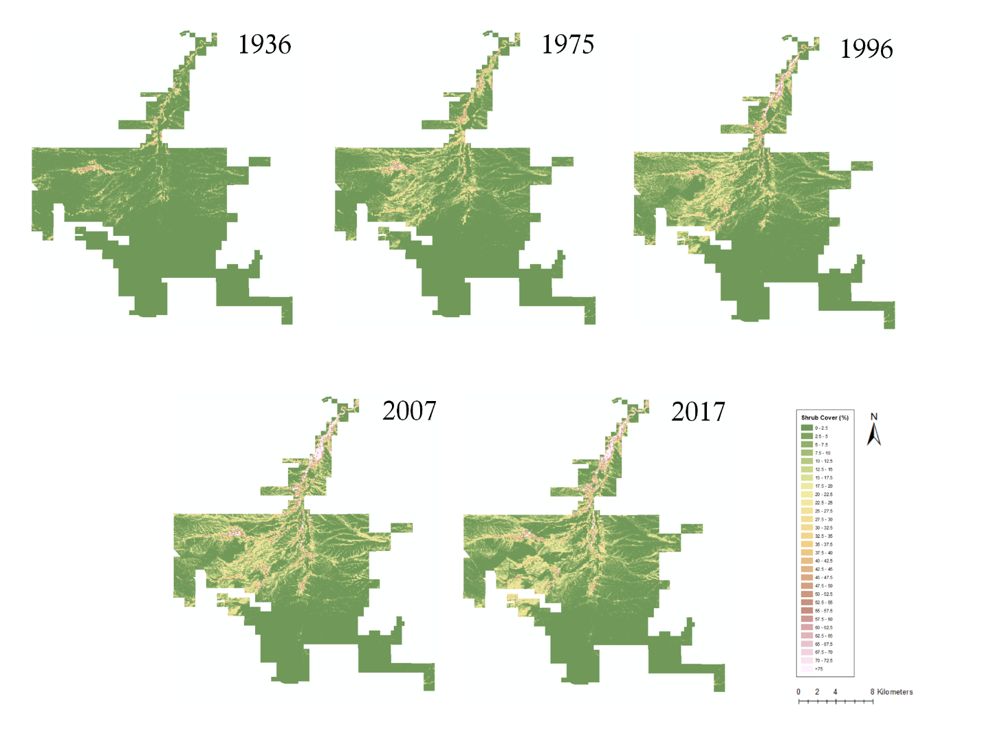
Aerial images used to classify shrub (primarily velvet mesquite [Prosopis velutina]) cover change across LCNCA ranged from 1936-2017 (Table 1). Images for years between 1950 and 1960 were not available.

Table 1. Date, scale, spectral type and source of images used in analysis of P. velutina encroachment. *The agency now known as the Natural Resource Conservation Service

Aerial photographs from 1936 were acquired from Arizona State University Map and Geospatial hub and scanned at 1200 dpi. All other images were downloaded in digital format from EarthExplorer (USGS; http://earthexplorer.usgs.gov/). To standardize differences in photo scale and resolution, all images were resampled to a common spatial resolution (1 m). Images for 1936 and 1975 were georectified to the 2017 orthorectified base image using ArcGIS (ESRI 2016).

An unsupervised image classification approach [Integrative Self-Organizing Data Analysis Technique (ISODATA)] was used. Where shrub canopies touched or overlapped it was not possible to reliably identify individual plants Accordingly, shrub “patches” were our classified sample units. One hundred classes were initially produced by the ISODATA classifications for each year. Classes were then manually assigned as “shrub” or “non-shrub” and reclassified. Region grouping and zonal geometry tools in ArcGIS were used to aggregate shrub patches into classes based on the number of 1-m pixels they covered. Entities smaller than 2 pixels (~ 2 m) created “salt and pepper” or speckled appearances to the output classified images and were omitted as it was uncertain whether this represented bunch grasses, succulents (Yucca spp., Opuntia spp) or small shrubs. To minimize shadow effects, poorly illuminated areas in the 1936 image were masked and omitted. These same areas were also omitted for all other years. Classification accuracies for each year were calculated using a point-based assessment (Stehman 2009), wherein random sample points (n =200) were stratified between “shrub” (n=100) and “non-shrub” (n=100) classes. Accuracies of these shrub cover maps were as follows:

2017: 94%, Kappa .88

2007: 96%, Kappa .90

1996: 90%, Kappa .80

1975: 92%, Kappa .84

1936: 84%, Kappa .69

Shrub cover was up-scaled from 1-m to 1-ha to buffer errors associated with georeferencing and resampling to a common resolution. Given the goal of quantifying shrub encroachment potential and response to brush management, areas with known disturbances (e.g. wildfire, human development, etc.) were masked and excluded from analyses. Areas where brush management practices had been conducted in past years were identified and excluded from analyses aimed at quantifying maximum shrub cover potential. Shrub cover change post-brush management were then compared to rates of cover change on undisturbed portions of the landscape (Figure 4).

Figure 4. Shrub cover (%) on the 42,000 acre Las Cienegas National Conservation Area in 1936, 1975, 1996, 2007 and 2017. Shrub cover was aggregated to 1-ha (100-m) to account for slight differences in georeferenced image positions.

Topo-edaphic template

Ecosites

We used an ecological site description (hereafter “ecosites”) map of LCNCA developed by the Natural Resource Conservation Service (NRCS; https://www.nrcs.usda.gov/wps/portal/nrcs/site/national/home/).

Topography

Elevation was obtained from a 1/3 arc-second (~10-m) digital elevation model (DEM) from the U.S. Geological Survey (USGS) National Elevation Dataset (https://www.usgs.gov/core-science-systems/ngp/tnm-delivery). Slope inclination and slope aspect were calculated from this DEM using the ArcGIS tools “Slope” and “Aspect”.

Soil Texture and Depth to Bedrock

Clay content was estimated using the global SoilGrids 2 map (Poggio et al. 2021) to represent soil texture at 0 (surface), 5, 15, 30, 60, 100 and 200 cm depths. Clay content in the surface and 5-cm depths was averaged and used as an index for infiltration potential. Depth to bedrock (max of 200 cm) was obtained from the SoilGrids platform (www.SoilGrids.org).

Topographic wetness index

A topographic wetness index (TWI; Sorensen et al. 2006) was used as an indicator of the effect of topography on soil moisture. TWI values for LCNCA were calculated using the TauDEM 5.0 software suite (Tarboton 2010).

Topographic wetness index

Statistical analysis

Topo-edaphic constraints on Maximum Shrub Coverage

The 95^th percentile of shrub cover was considered the maximum potential shrub cover. Quantile regression (Koenker et al. 1994) was used to characterize the effects of topo-edaphic constraints (elevation, soil texture, slope inclination, slope aspect and TWI) on the maximum potential shrub cover on a given site using the 2017 shrub cover map with the assumption that shrub cover should have reached its maximum cover potential over the past century of encroachment. Quantile regression was chosen over other regression methods (i.e. linear, least square and mean) due to its ability to buffer the influence of outliers such as those caused by unaccounted for past disturbances (Cade & Noon 2003). Linear quantile regressions were first calculated using the ‘rq’ function within the ‘quantreg’ library in R (http://r-project.org/) for each variable across the entire study site and then specific to the six ecosites comprising ~94% of the LCNCA land area. If the slope a linear quantile regression was found to be significantly different from zero, a second quantile regression was run using the ‘segmented’ R package (Muggeo, 2008) to model interactions using breakpoint analysis.

Topo-edaphic influence on Shrub Coverage Change

Boosted Regression Trees (BRTs) were used to assess interactions among the variables listed above and shrub cover change. BRTs are a form of machine learning that iteratively fit and combine multiple regression tree models to improve predictive performance. BRTs were fitted in R using the ‘dismo’ package per Elith et al. (2008).

A terrain ruggedness index (sum change in elevation between pixels in the DEM) and additional edaphic data obtained from the SoilGrids 2 platform were also used to model shrub cover change. These additional soil variables included bulk density (kg m³), cation exchange capacity (cmol kg⁻¹); soil organic carbon content (g kg⁻¹), total nitrogen (cg/kg) and pH (in H₂O). Values for shrub cover change values were calculated per 100x100m pixels by subtracting shrub cover values in 1936 by 2017 cover values.

Objective 3: Model Spatiotemporal Ecosystem Service Capacity

With the completion of shrub cover layers for created in Objective 2, modeling of spatial temporal ecosystem services has begun. This portion of the project will continue and is slated for completion in during the 2021/2022 academic year.

Research results and discussion:

Objective 1: Preliminary Results

Image-based analysis

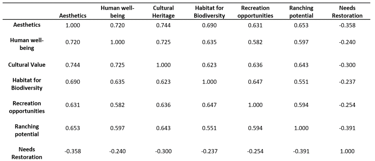
Of the 103 responses received as of this writing, 15 (14.5%) were residents and recreationalists, 19 (18.5%) were non-profit/non-governmental, 16 (15.5%) were ranchers/producers, 29 (28.2%) were governmental/land managers, and 24 (23.3%) were academicians. Correlation analysis found the two strongest-correlated variables were (i) aesthetics and cultural heritage (Spearman’s rho = 0.744, p < 0.001) and (ii) human well-being and cultural heritage (Spearman’s rho = 0.725, p < 0.001). Habitat for biodiversity best correlated with aesthetics (Spearman’s rho = 0.690, p < 0.001). Recreational opportunity was correlated strongest with habitat for biodiversity (Spearman’s rho = 0.647, p < 0.001) and ranching potential was correlated with aesthetics (Spearman’s rho = 0.653, p < 0.001). Need for restoration practices was correlated highest with ranching potential (Spearman’s rho = -0.391, p < 0.001) and lowest with habitat for biodiversity (Spearman’s rho = -0.237, p < 0.001) (Table 2).

Table 2. Spearman correlations’ coefficients (Spearman’s rho) between the seven benefits evaluated in this study: aesthetics, human well-being, habitat for biodiversity, cultural heritage, recreation opportunities, ranching potential, and requiring restoration.

Post-hoc Tukey tests indicated that respondents identified most positively with images depicting lower shrub cover with mean ranking scores dropping as shrub cover increased (Figure 5). An exception to this was biodiversity which was statistically similar (Tukey’s post-hoc tests) across all images except Image 7 (highest cover). Insights from an optional explanation section within the survey suggests that respondents did not view biodiversity as a net-loss with encroachment. Instead, it was perceived that while some grassland specialist species may be negatively impacted, some generalist species would benefit from higher shrub cover.

Best-worst Scaling

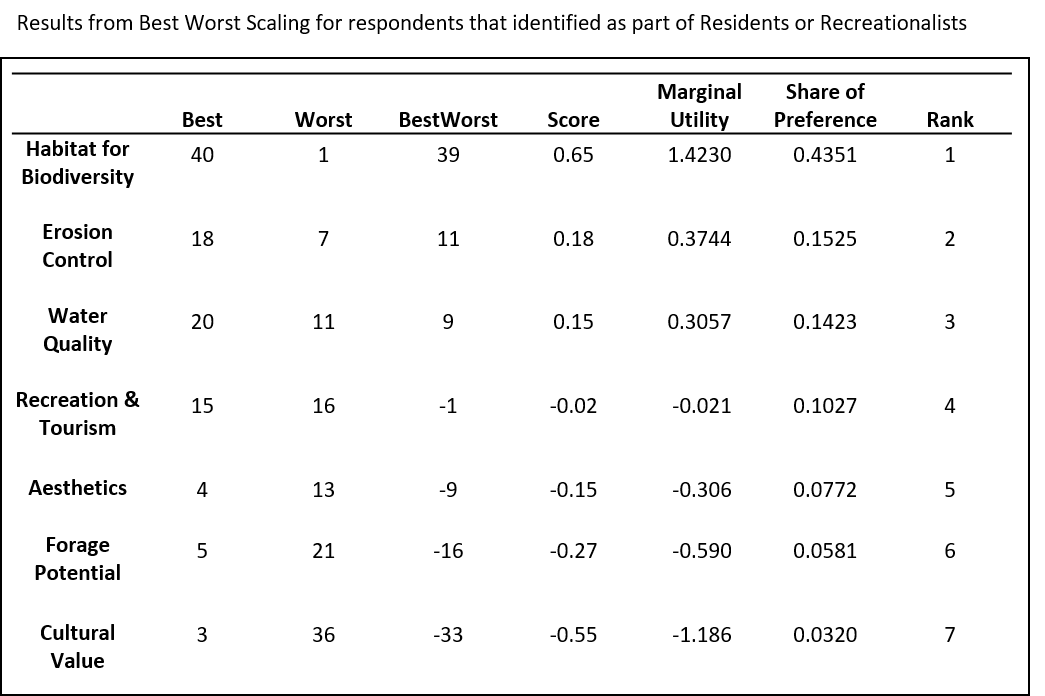
Habitat for biodiversity was ranked highest by participants (BW score = 0.68) followed by erosion control (BW = 0.43) and water quality (BW = 0.25) (Table 3). Aesthetics, cultural value, recreation and tourism, and forage potential all received negative scores which mean those services were identified as the “worst” option more often than being chosen as the “best” option. Aesthetic value ranked lowest (BW = -0.38).

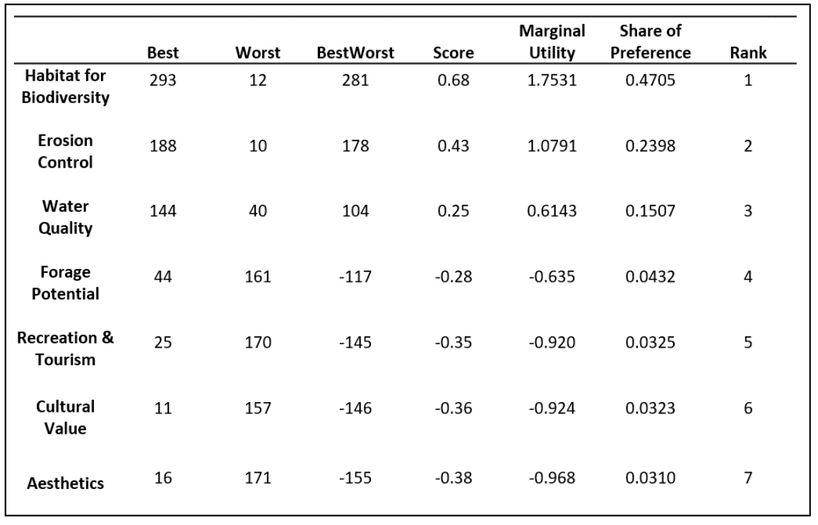
Table 3. Frequency each service selected as the Best and Worst reason to conserve or restore desert grasslands as well as the “shared preference” for each service. Marginal utility is an indicator of the perceived value of the corresponding level of the effect. Larger scores are indicators of the relative value placed on a given service.

A conditional logit was used to estimate the “shared preference” for each ecosystem service which is an indication of the probability that a respondent showed a preference for one service over all others (Table 3). Results indicate that habitat for biodiversity, which was ranked highest amongst respondents, was approximately 15 times ( = 0.4705/0.0310) more important than the lowest ranked service cultural heritage and 2 times ( = 0.4705/0.2398) more important than the second highest-ranked service erosion control.

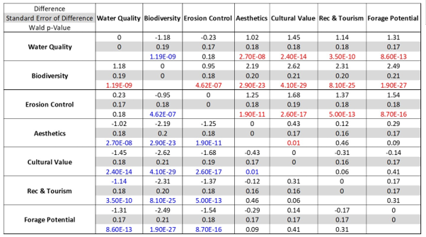
Specific comparisons between services can further be seen in the All-Variable Comparison Report (Table 4). For example, erosion control was found to have a significantly higher preference among respondents than aesthetics, cultural value, recreation & tourism, and forage production but was less preferable than habitat for biodiversity and statistically comparable to water quality.

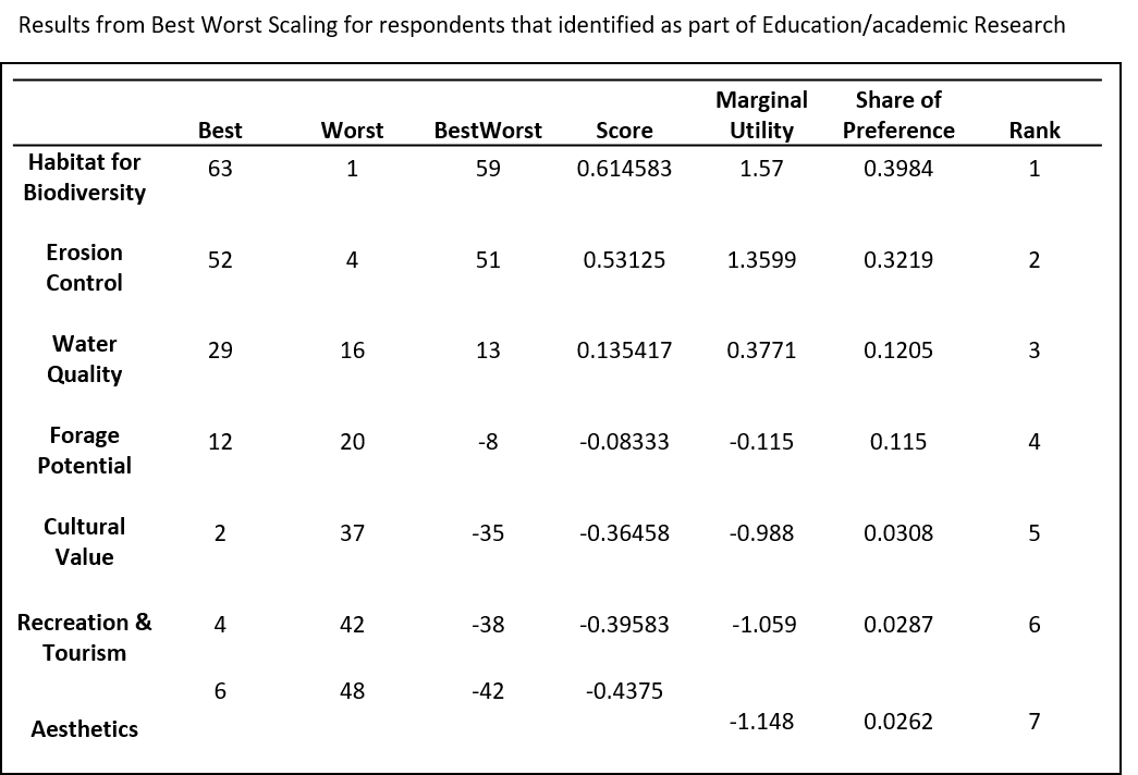
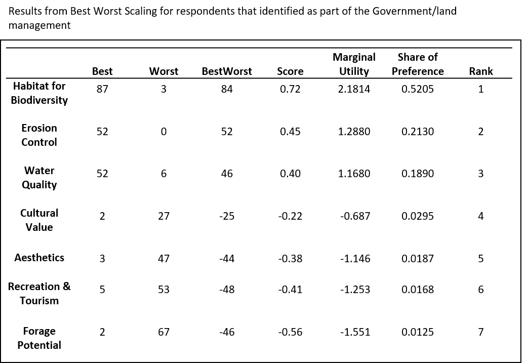
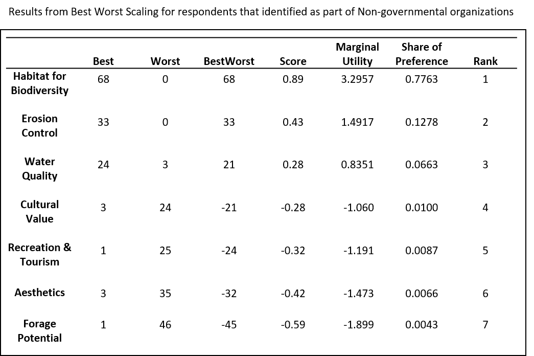
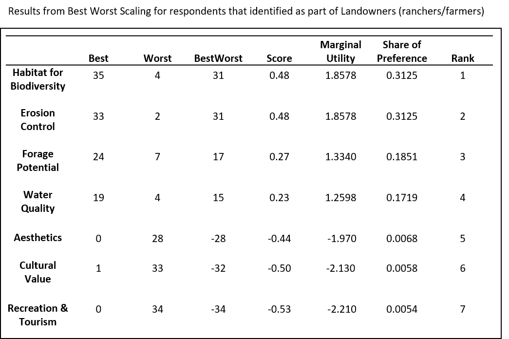
Table 4. All-Variables Comparison Report for the seven ecosystem services evaluated in this study. Each comparison is the difference in preference between the ecosystem service type in the row and the service in the column. Statistically significant values (p < .05) are colored either blue or red depending on the sign (+/-) of the difference.

Similar Best-Worst Scaling methods were applied to participants based on their stakeholder affiliation (Table 5). Habitat for biodiversity and erosion control were selected as the first and second most important ecosystem services across all stakeholder groups. Water quality was the thirst most important service across all groups outside of ranchers/landowners who ranked forage potential as the third highest service with a score of .27. Rancher and landowner placement of ranching potential contrasted with the other groups who ranked this service lower and with a negative score. For academics, forage potential was ranked 4^th (score = .08) while both governmental (score = -.56) and NGO (score = -.59) stakeholders ranked this service lowest. Results of each stakeholder groups BWS results are summarized in Tables 6-10.

Table 5. Ecosystem services displayed by order of decreasing relative importance by stakeholder group.

Table 6. Frequency of services selected as the “Best” and “Worst” reason to conserve or restore desert grasslands for the education/academic stakeholder group as well as the “shared preference” for each service. “Marginal Utility” is an indicator of the perceived value of the corresponding level of the effect. Larger scores are indicative of greater relative importance.

Table 7. Frequency of services selected as the “Best” and “Worst” reason to conserve or restore desert grasslands for the government and land management stakeholder group as well as the “shared preference” for each service. “Marginal Utility” is an indicator of the perceived value of the corresponding level of the effect. Larger scores are indicative of greater relative importance.

Table 8. Frequency of services selected as the “Best” and “Worst” reason to conserve or restore desert grasslands for the non-profit/non-governmental stakeholder group as well as the “shared preference” for each service. “Marginal Utility” is an indicator of the perceived value of the corresponding level of the effect. Larger scores are indicative of greater relative importance.

Table 9. Frequency of services selected as the “Best” and “Worst” reason to conserve or restore desert grasslands for the landowner (rancher/farmer) stakeholder group as well as the “shared preference” for each service. “Marginal Utility” is an indicator of the perceived value of the corresponding level of the effect. Larger scores are indicative of greater relative importance.

Table 10. Frequency of services selected as the “Best” and “Worst” reason to conserve or restore desert grasslands for the residence and recreationalist stakeholder group as well as the “shared preference” for each service. “Marginal Utility” is an indicator of the perceived value of the corresponding level of the effect. Larger scores are indicative of greater relative importance.

Objective 2:

Shrub cover change across LCNCA

Shrub cover at the 1-ha scale varied greatly across the study site with total shrub cover across the entire site steadily increasing over the past 81 years (1.6% in 1936, 2.8% in 1974, 4.1% in 1996, 5.8% in 2007 and 6.1% in 2017).

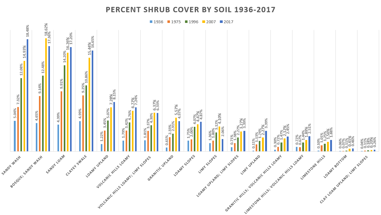
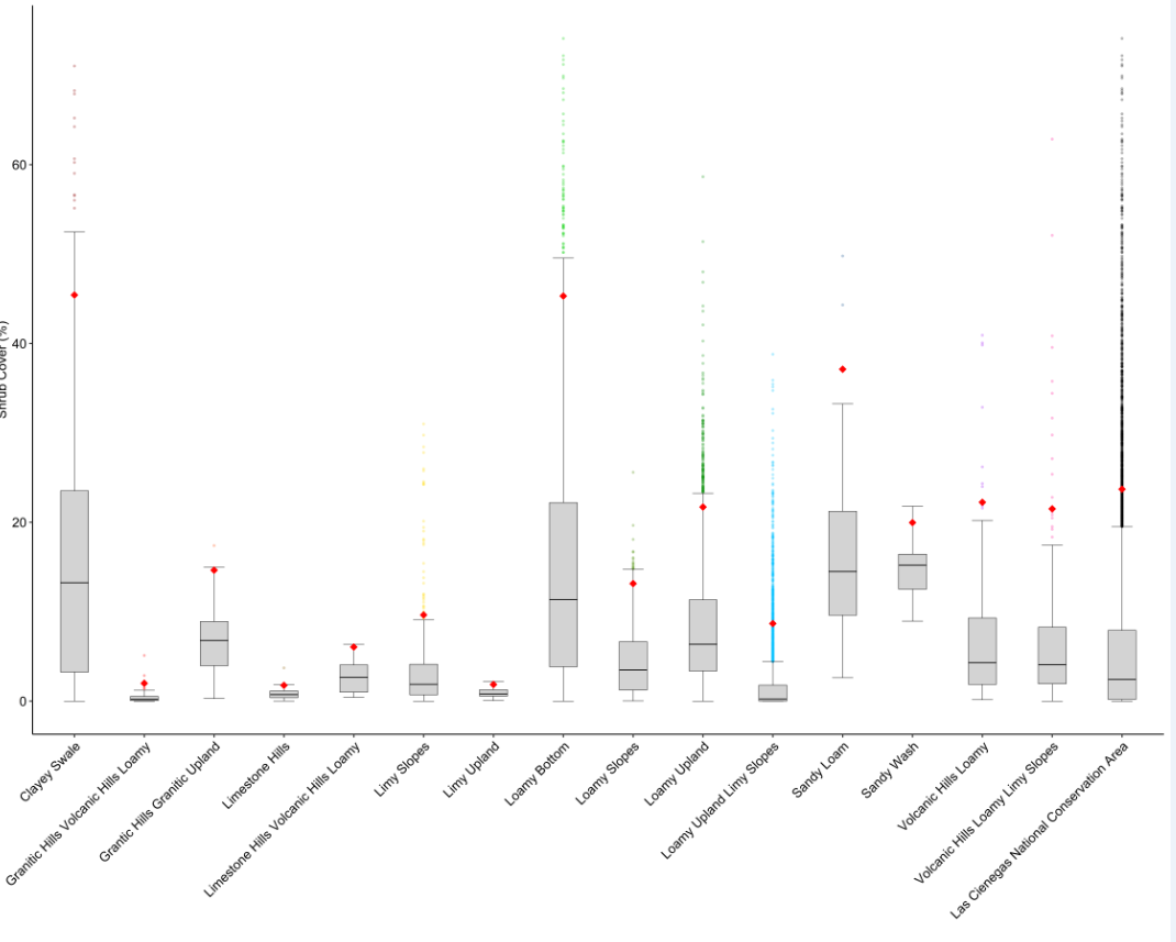
Figure 6. Shrub canopy cover (%) from 1936-2017 on contrasting upland soil types (areas of past brush management and sites within 100 m of drainages omitted).

Shrub cover on the various soil types (excluding intermittent drainages and areas subject to past brush management) ranged from 0.04% to 5.04% in 1936, 0.11% to 9.91% in 1975, 0.18% to 14.20% in 1996, 0.20% to 18.62% in 2007 and 0.26% to 18.48% in 2017 (Figure 6). Sandy washes, sandy loam, and clayey swales had the highest initial coverage and experienced the greatest subsequent increases in shrub cover. Clay loam upland, limy slopes and loamy bottoms had the lowest initial shrub cover and also experienced lowest levels of subsequent encroachment.

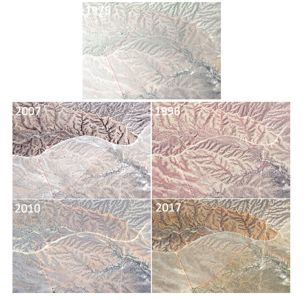
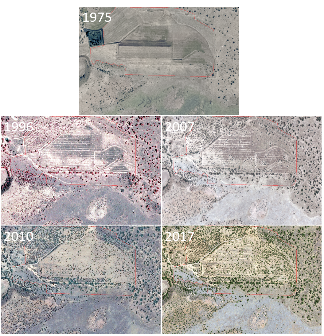
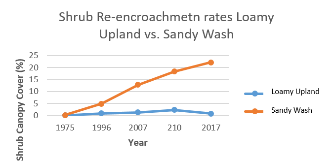
Post brush management re-encroachment

Areas in LCNCA that have undergone past brush management were mapped and analyzed to assess rates of shrubs re-establishment. Because aerial imagery is more readily available beginning in the 2000s, additional National Agricultural Imagery Program (NAIP) years have been included for these analyses. Two examples, a loamy upland site and a sandy wash site are shown in Figures 7 and 8. Both were mechanically cleared in the 1970s and in 1975 both had < 1% shrub cover. Re-establishment rates on these sites varied greatly as the loamy upland saw shrub canopy cover increase to 2.3% in 2010 at which time re-treatment brought cover to < 1% in 2017. Re-establishment was more rapid on the sandy wash sites, reaching 18.4% by 2010 and 22.1% by 2017 (Figure 9). These results will be valuable for land managers as they provide a basis for understanding on how shrub re-establishment rates are controlled by topo-edaphic factors and projecting when a follow-up treatment may be required to meet a given management objective.

Figure 7 Loamy upland site that underwent mechanical brush management in the 1970s with follow-up treatment occurring in 2010. Fire occurred in this area in 2007 but was not found to have an effect on larger shrubs.

Figure 8 Sandy wash site that was a shrub-free agricultural field prior to 1975. Fields were subsequently abandoned, thus opening the door for shrub encroachment.

Figure 9. Post-treatment re-establishment of shrub cover on a loamy upland and sandy wash ecological sites. Both sites were mechanically cleared of shrubs in the early 1970s. The loam upland site was re-treated in 2010.

Shrub encroachment and topo-edaphic constraints

Linear and additive non-parametric quantile regression analysis was used ascertain the potential upper limit of shrub cover (95^th percentile) for a given topo-edaphic settings. Shrub cover values across all years were aggregated for these analyses with the assumption that the 95^th percentile approximates the upper limit of shrub cover in that location.

Ecosites

Pooled across LCNCA ecosites the upper limit of shrub cover or “shrub cover potential” was 17.6%. Shrub cover potential was highest on loamy bottoms (37.4%) and clayey swales (35.8%) and lowest on granitic hills volcanic hills loamy (2.0%) and limestone hills (1.8%)(Figure 10). The two most spatially extensive ecosites on the LCNCA, loamy uplands (4,919 ha) and loamy uplands limy slopes (6,734 ha) had shrub cover potentials of 5.4 and 16.6%, respectively. This difference is believed to reflect elevation-effects.

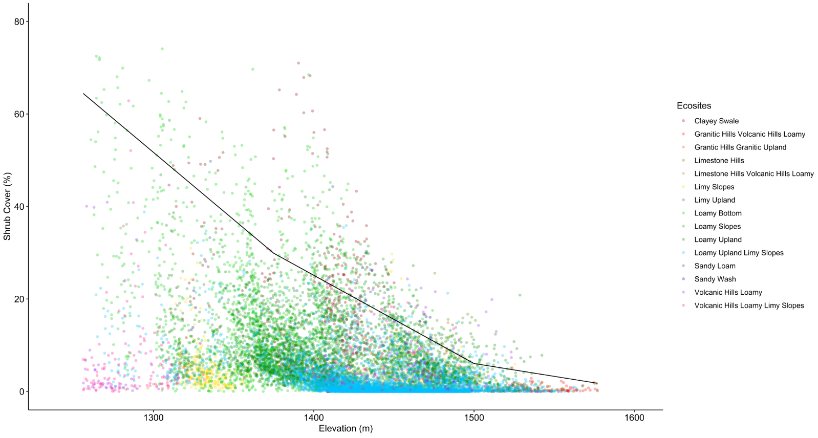
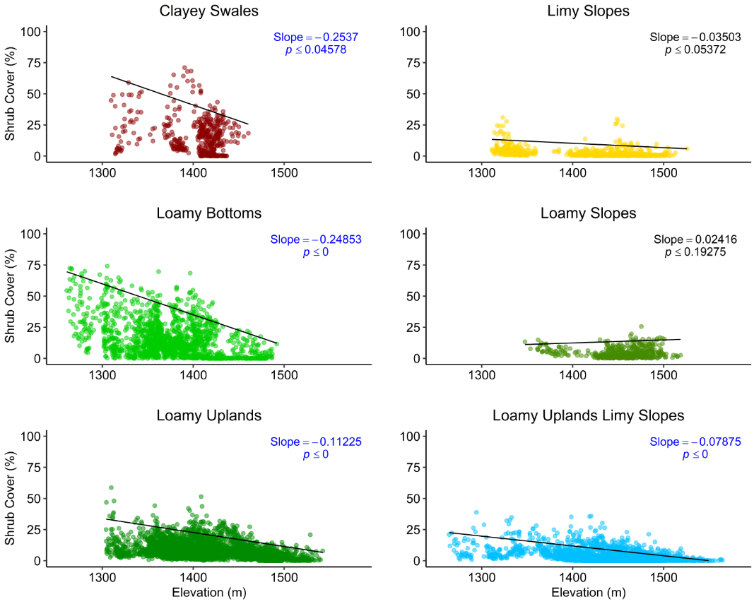
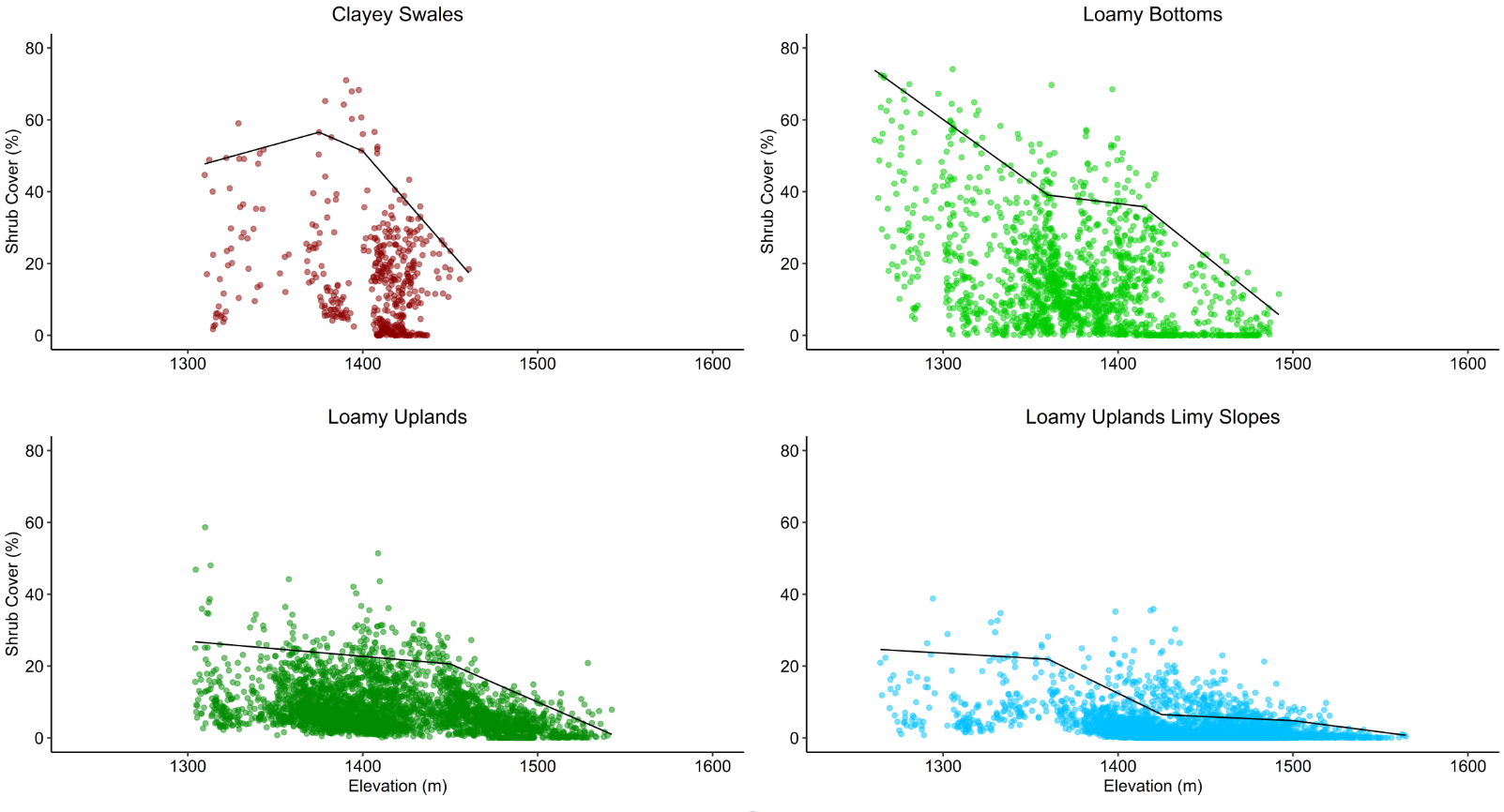
Figure 10. Box and whisker plots of shrub cover (%) by ecosite. The center, bottom, and top of boxes indicate the median, the 25th percentile, and the 75th percentile; red diamonds are the 95th percentiles.

Elevation

Within the LCNCA, the upper limits of shrub cover potential was found to decrease with increasing elevation: as elevation increased from 1360-m to 1465-m potential shrub cover decreased from 56% to 9%. From 1465-m to the max elevation of 1572-m potential shrub cover stayed relatively steady with only a slight decrease from 9% to 4% (Figure 11). Linear quantile slopes were significantly different than zero for clayey swales, loamy bottoms, loamy uplands, and loamy uplands limy slopes ecosites; slopes for limy slopes and loamy slopes were not found to be significant (Fig. 12). Breakpoint segmented quantile regressions (Figure 13) indicated that shrub cover potential decreases as elevation increases.

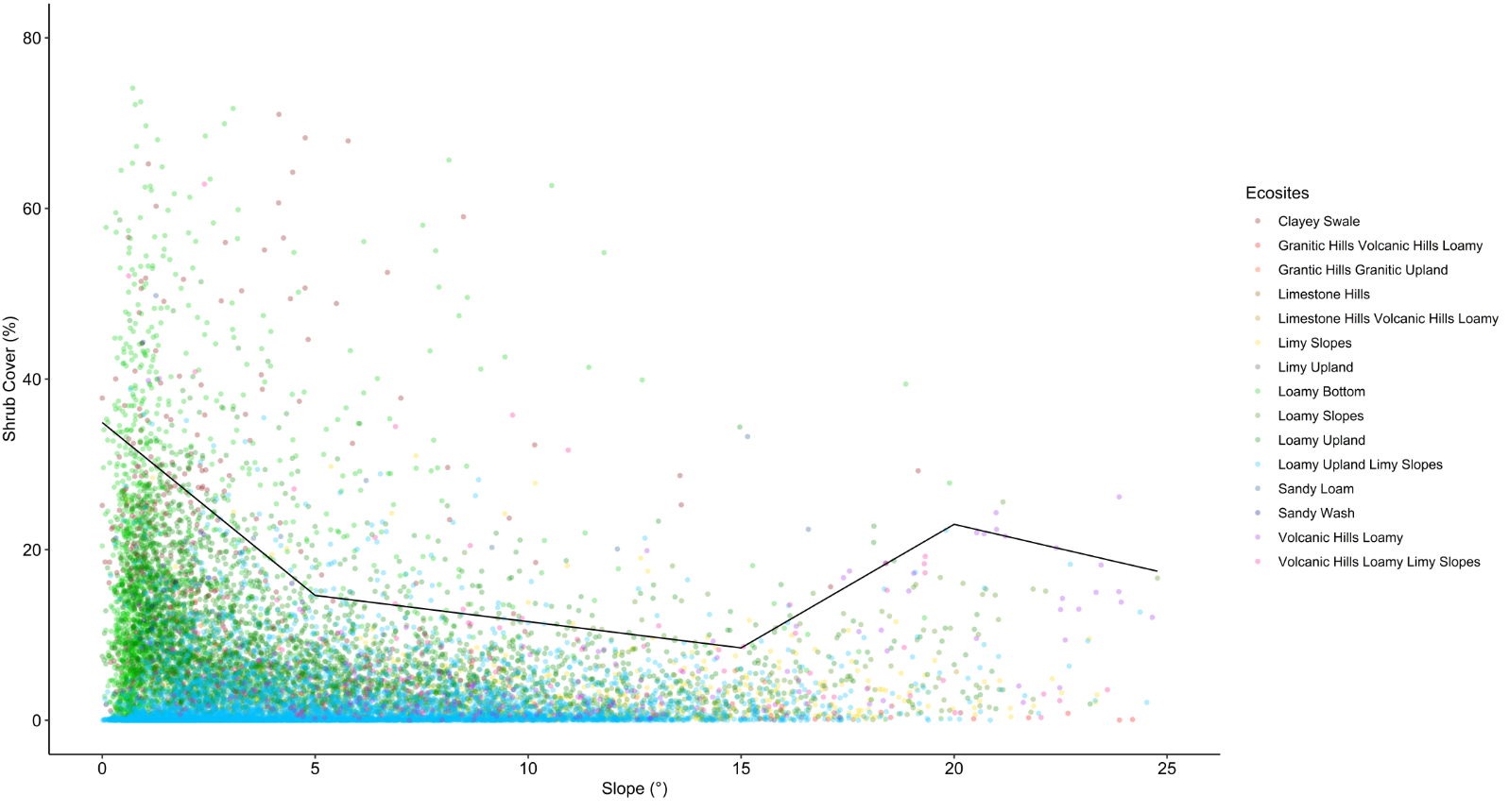
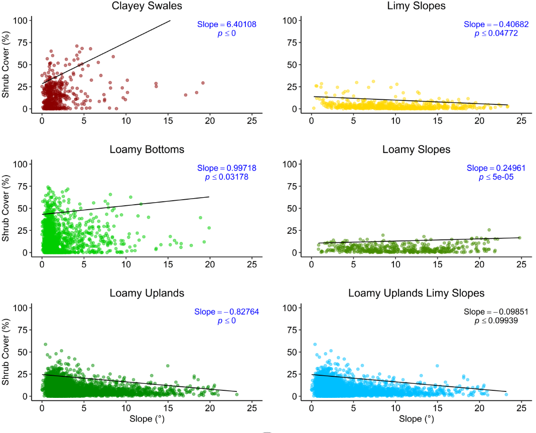
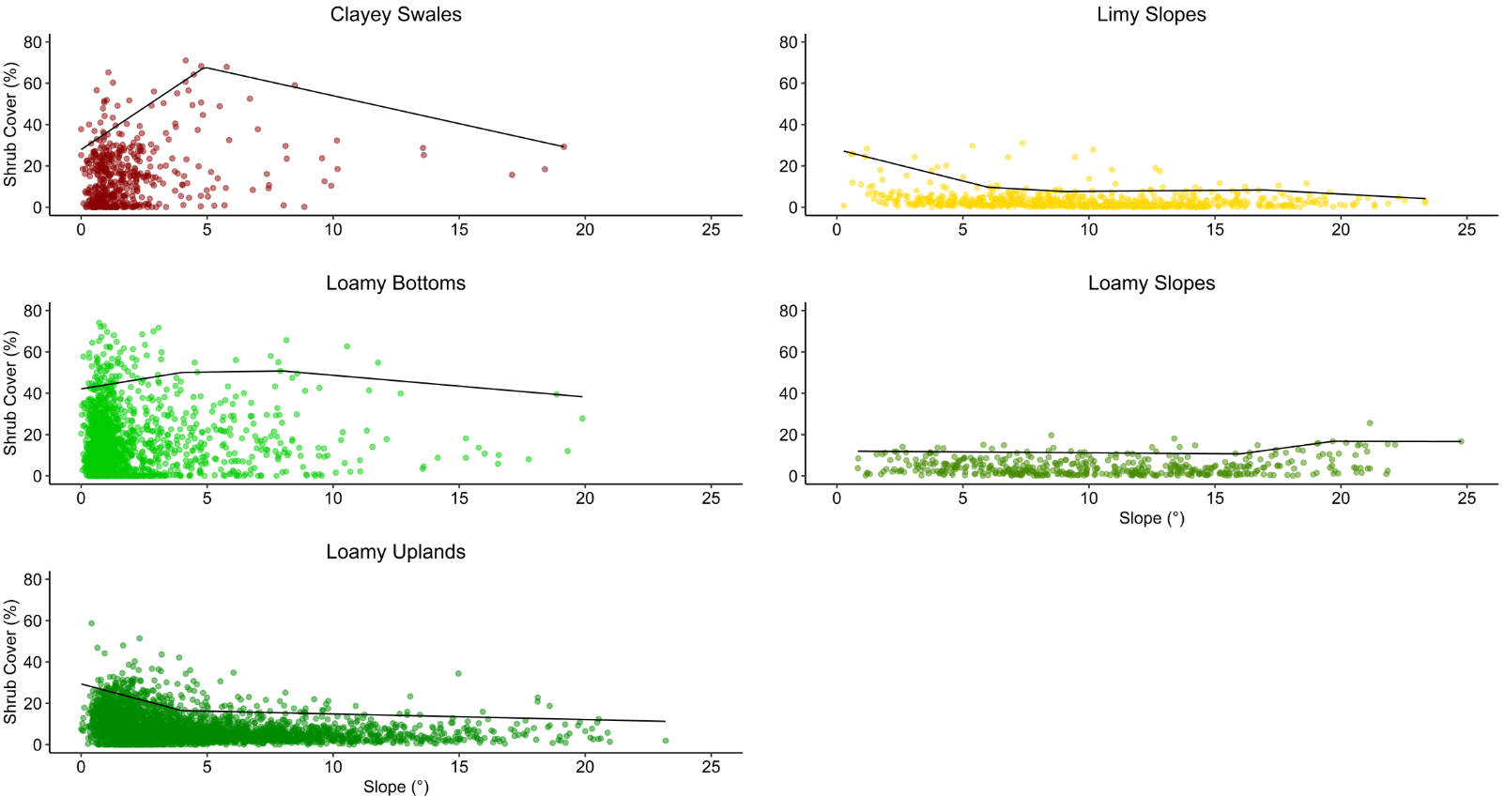
Figure 12: Linear quantile regression results for shrub cover (%) by elevation (m) for the six major ecosites at LCNCA. Black lines represent the 95th quantile regression line. Slope values in blue were statistically different from 0; those in black were not.

Figure 13: Segmented quantile regression results of shrub cover (%) by elevation (m) for ecosites whose linear quantile regression slope were significantly different from zero. Black lines represent the 95th segmented quantile regression line. Shrub cover potential for each of these ecosites decreased with increases in elevation.

Slope inclination

Upper limits of shrub cover across LCNCA had a ‘U-shaped’ relationship with slope inclination with potential maximum cover decreasing up to ~ 15°, at which point potential cover increased as slope steepness increased (Figure 14). With the exception of loamy uplands limy slopes shrub cover was statistically influenced by slope inclination (Figure 15). Unlike elevation, this relationship differed among the major ecosites with both loamy bottoms and clayey swales showing increases in cover potential as slope increased. Loamy uplands and limy slopes were found to have an initial drop in potential cover which then leveled off (Figure 16).

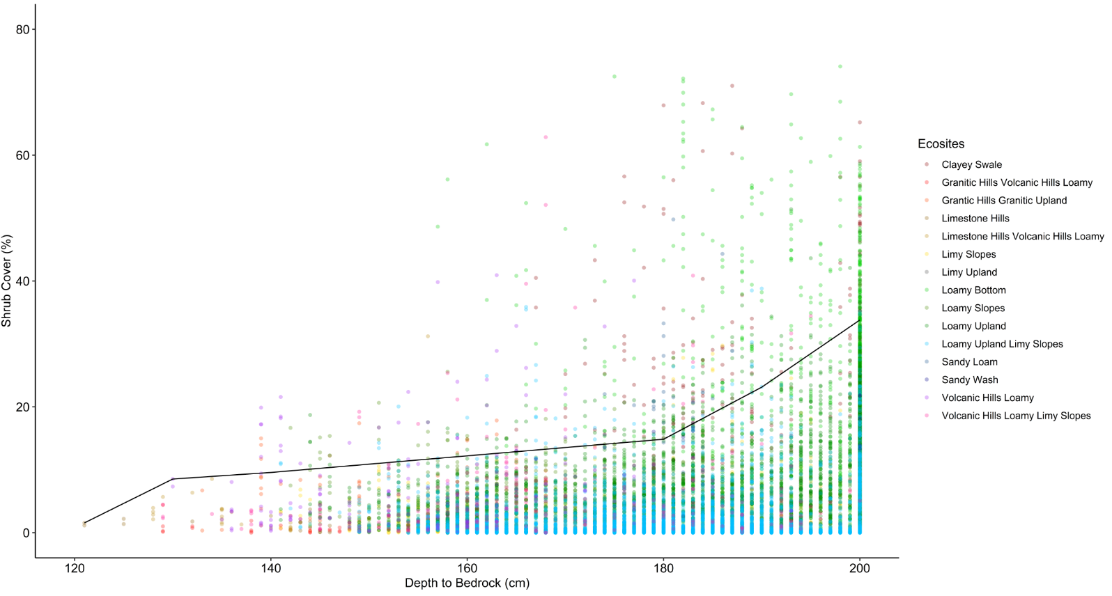
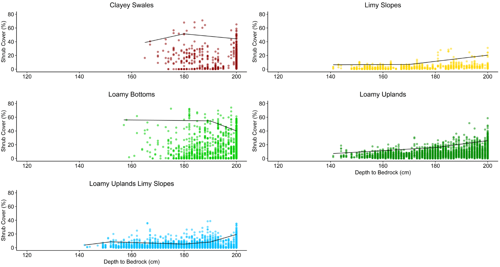
Figure 15: Linear quantile regression results for shrub cover (%) by inclination (degrees, °) for the six major ecosites at LCNCA. Black lines represent the 95th quantile regression line. Slope values in blue values were found to be statistically different from zero; those in black were not.

Figure 16: Segmented quantile regression results of shrub cover (%) by slope inclination (degrees, °) across major ecosites at LCNCA. Only ecosites whole linear quantile regression slope was found to be statistically different from zero are shown. Black lines represent the 95th segmented quantile regression line. Shrub cover potential for each of these ecosites was found to decrease with increases in slope inclination.

Depth to Bedrock

Across LCNCA, maximum shrub cover potential increased as depth to bedrock increased (Figure 17). It is hypothesized that this may be due to the competitive advantage deep rooting shrubs, gain over grasses. Accordingly, shrub cover potential is higher in areas where water can pernitrate deeper into the soil. Across the major ecosites, loamy bottoms, limy slopes, loamy uplands, and loamy uplands limy slopes were found to have significant interactions with depth to bedrock (Figure 18). Interestingly, both loamy bottom and clayey swales ecosites were found to have shrub cover potential decrease as depth to bedrock increases while limy slopes, loamy uplands, and loamy uplands limy slopes saw shrub cover potential increase (Figure 19).

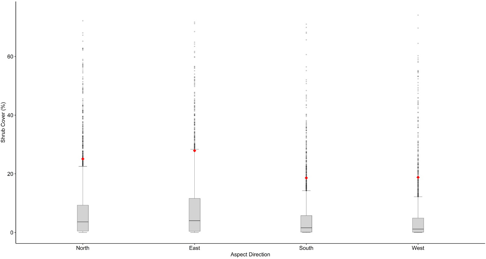
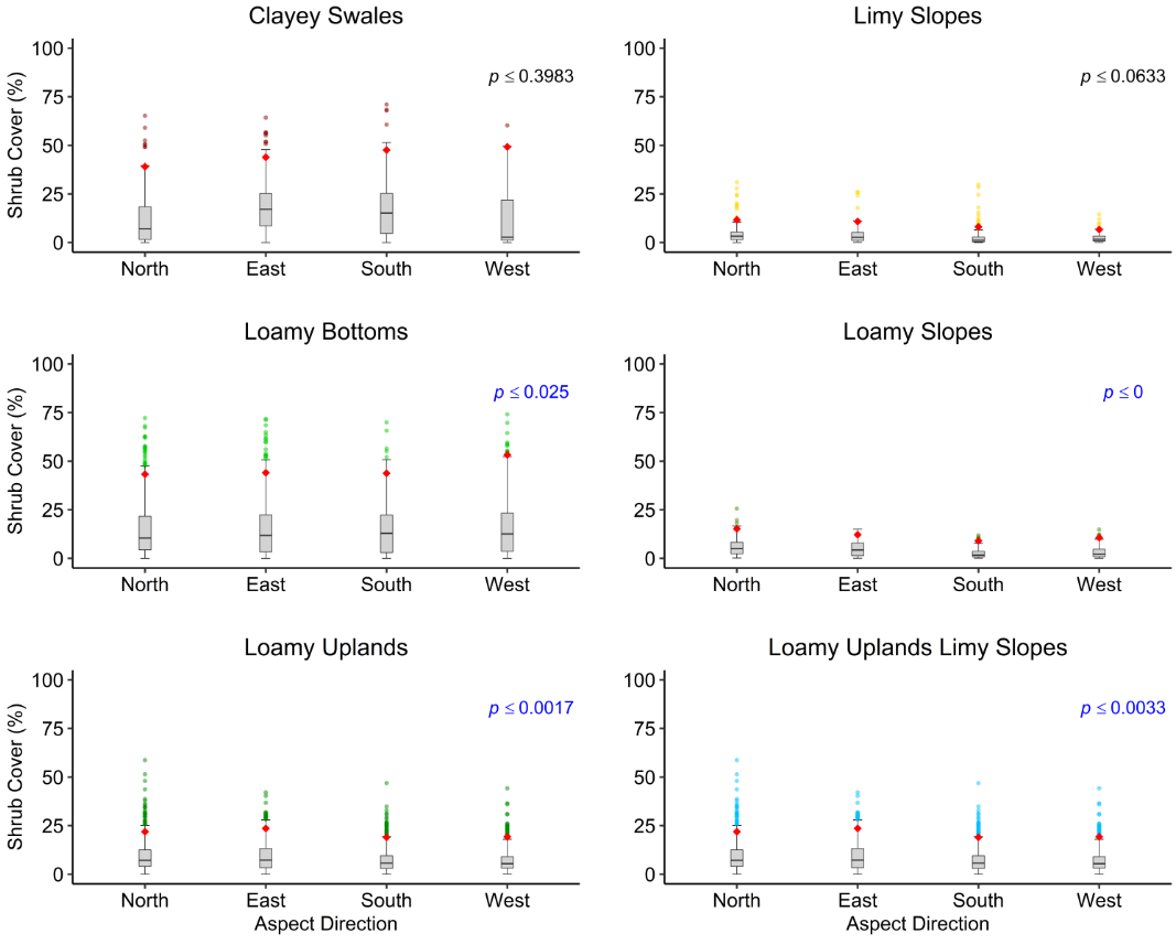
Figure 18: Linear quantile regression results for shrub cover (%) by depth to bedrock for the six major ecosites at LCNCA. Black lines represent the 95th quantile regression line. Slope values in blue values were statistically different from zero; those in black were not.

Figure 19: Segmented quantile regression results of shrub cover (%) by depth to bedrock across major ecosites at LCNCA. Black lines represent the 95th segmented quantile regression line. Shrub cover potential for each ecosite decreased with increases in depth to bedrock.

Slope aspect

Potential shrub cover was found to be highest on East- (27.9%) and North- (25.1%) facing slopes and lower on South- (18.6%) and West- (18.8%) facing slopes (Figure 20). On loamy bottoms shrub cover potential was highest on West- (53.2%) facing slopes and lower and relatively similar across other aspects; North- (43.3%), East- (44.1%) and South- (43.7%). For loamy slopes, loamy uplands and loamy uplands limy slopes potential cover was highest on North and East facing slopes and lowest on South and West facing slopes. Potential shrub cover was not significantly different across clayey swales and limy slopes (Figure 21).

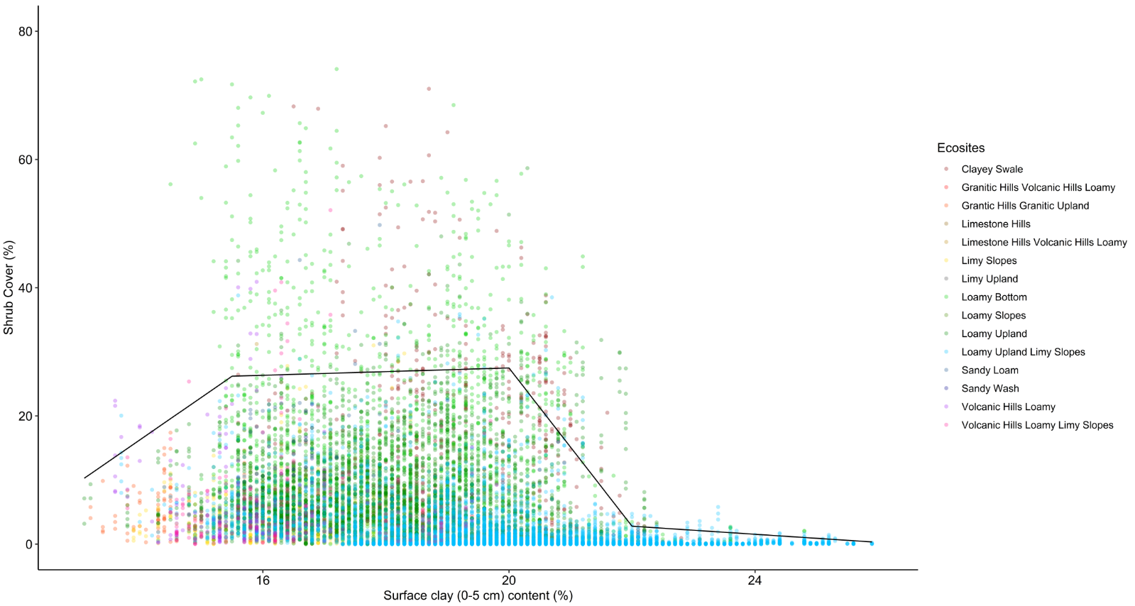
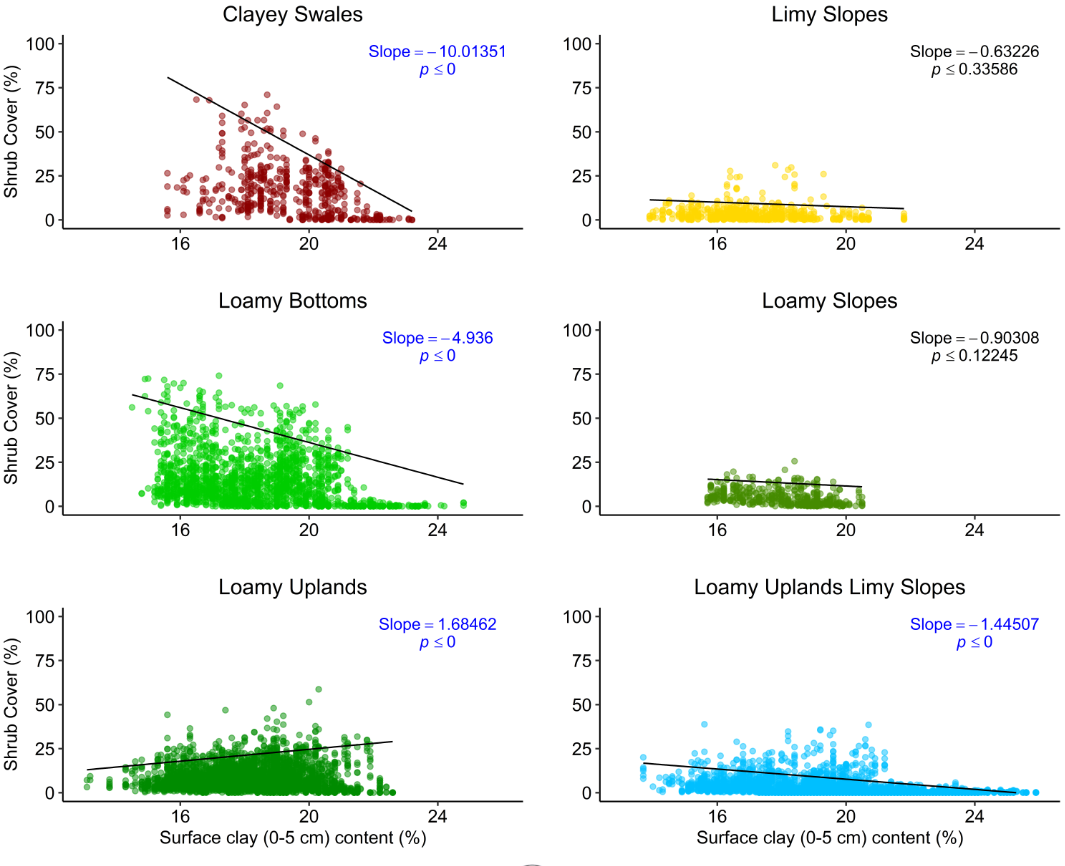
Figure 21. Box and whisker plots of shrub cover (%) in relation to slope aspect on the major ecosites at LCNCA. The center, bottom, and top of boxes indicate the median, the 25th percentile, and the 75th percentile; diamonds are the 95th percentiles. P-values in blue denote statistical differences <0.05.

Surface Clay (0 – 5cm)

Soil texture is believed to influence potential shrub cover due its effects on precipitation infiltration/percolation and soil fertility. Soils with high clay content may be more resistant and sandy soils more susceptible to shrub encroachment. These trade-offs were observed based on shrub cover potential and surface clay content across LCNCA (Figure 22). As surface clay increased from 13% to 16% potential shrub cover increased to ~23% and stayed stable until 20% clay content whereupon cover declined. At >23% clay content shrub cover was low and stable.

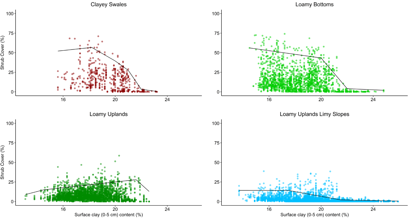
Figure 22: Shrub cover (%) as a function of surface (upper 5-cm) clay content. Data points are color coded by ecosites (see above key). Black line represents the 95th quantile regression line.

This relationship was similar across the major ecosites at LCNCA with clayey swales, loamy bottoms, loamy uplands and loamy uplands limy slopes all showing a marked declines in shrub cover potential when clay content exceeded 21% (Figure 23).

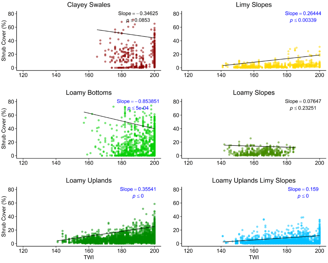
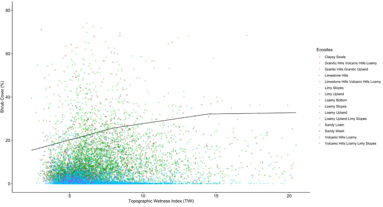
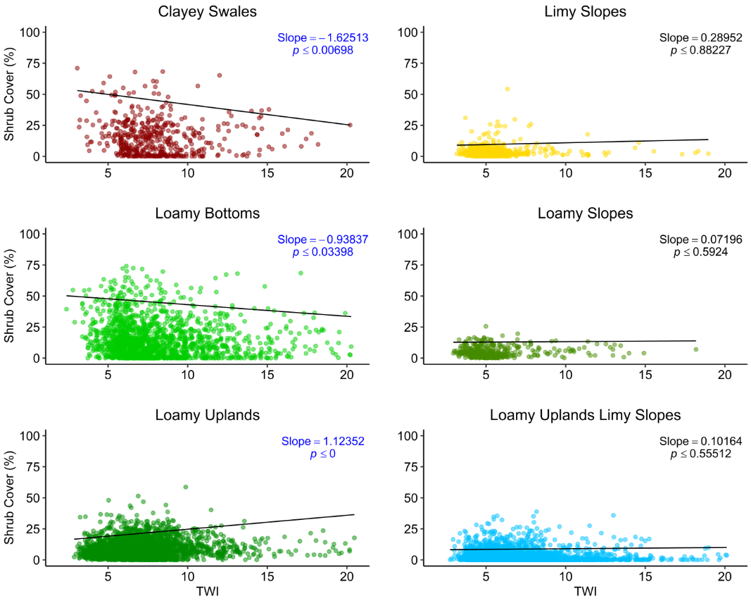
Figure 23: Segmented quantile regression results of shrub cover (%) as a function of surface (upper 5-cm) clay content on major ecosites at LCNCA. Black lines represent the 95th segmented quantile regression line.

Topographic Wetness Index (TWI)

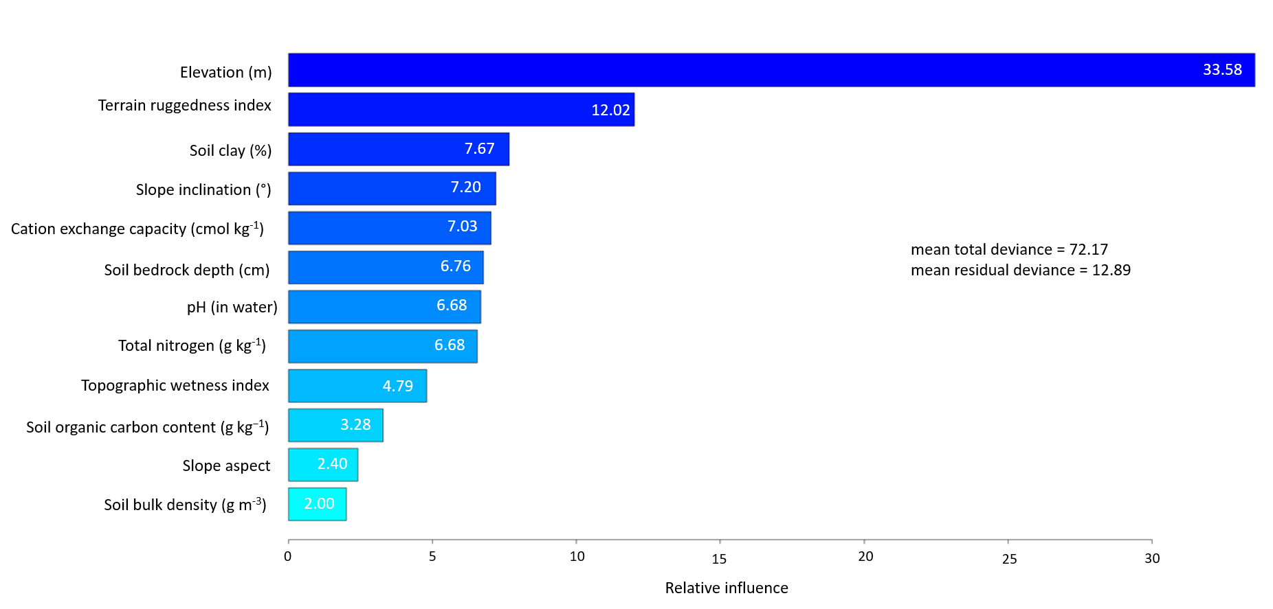
A total of 5,000 individual regression trees were created in the final boosted regression tree (BRT) model with explanatory variables explaining 72% of the total variance in shrub cover change. Of these variables, elevation (33.6% relative importance) overwhelmingly had the greatest influence on predicting shrub cover change (Fig. 26). The topographic ruggedness index had the second highest influence (12% relative importance). Surface clay content, slope inclination, cation exchange, mean soil pH and mean soil nitrogen all had similar importance values of ~7%. Soil organic carbon, slope aspect direction, had the least influence (<4%).

Topo-edaphic influence on Shrub Coverage Change

Figure 26: Relative contribution (%) of the explanatory variables in the Boosted Regression Tree (BRT) model. The model explained 73% of the total variance in shrub cover change.

Participation Summary

29 Producers participating in research

Research Outcomes

No research outcomes

Education and Outreach

3 Tours

12 Webinars / talks / presentations

2 Workshop field days

Participation Summary:

29 Farmers participated

108 Ag professionals participated

Education and outreach methods and analyses:

Participation Summary

To date, 18 participants have been directly involved in the study through semi-structured interviews as well as 108 participants who completed the online survey. Participants include academicians, government employees, non-government personnel, and land users. Numerous other stakeholders from the above list have been involved though informal interviews/ conversations or site visits to show and explain shrub encroachment/brush management at LCNCA or other similar sites in Southern Arizona. For example, in November 2019 I took a team of 8 visiting French researchers to LCNCA to show them results of different brush management projects conducted on different sites. In April 2021 I met with ranchers in the Altar Valley to discuss current brush management projects and participated in discussions on planning future follow up treatments. I am scheduled to make a presentation at the summer meeting of the Arizona Section of the Society for Range Management (August ??, 2021) that will be attended by Cooperative Extension agents, land managers with County, State and Federal agencies, and producers.

Outreach & Education Description

2019-2021

On April 1, 2021 I deliver a “lunch and learn” presentation (~1 hour) to members of the Cienega Watershed Partnership. This event was attended by a broad diversity of people (~ 45), many of whom had only a superficial knowledge or understanding of shrub encroachment/brush management. A number of researchers who are active in planning conservation actions within the Cienega Watershed were also present and very interested in this projects results as it has direct implications and information to planned restoration activities.

At this year’s virtual Society for Range Management Annual Meeting I presented a poster on February 15, 2021 covering results from Objective 1. Due to COVID concerns forcing this conference to be held virtually interactions were challenging. With that said, some good discussions did occur – especially with how to increase stakeholder participation and inclusion of diverse groups within projects like this one. I was also contracted directly by five people who wanted to be kept updated on results as they emerge.

A poster presentation on Objective 2 was given February 18, 2020 at the annual meeting of Society for Range Management in Denver, Colorado. This national/international conference draws a diverse set of participants including research scientists, governmental and non-governmental land managers, and producers. I was able to interact with a number of people during my poster session. Discussions ranged from GIS/Remote sensing methods for classifying historical imagery, acquisition of historical imagery, and perspectives (professional and anecdotal) on drivers of shrub encroachment.

2018-2019

A 30-minute oral presentation was given at the June 22, 2019 Science on the Sonoita Plain Symposium in Elgin, Arizona (http://www.cienega.org/event/sosp-10th-annual-symposium/). The conference was attended by ~50 participants and included scientists, governmental and non-governmental land managers, producers, and interested local citizens. The presentation generated good discussion and interest as many people saw connections of how this work can be applied to ongoing and planned activities in the region. Participants were interested in my research might help better plan best places to treat and when to plan for retreatments. From this, I was able to provide shrub cover maps for the allotted treatment areas spanning from 1936 to present. These maps are being used by the lead brush treatment manager to target which sites are best suited for treatment (i.e. has underdone significant encroachment vs. high shrub cover always present) as well as logistics of the treatment themselves.

A poster presentation of Objective 2 results was made on December 4, 2018 at the University of Arizona’s Fall Student Showcase. The poster was presented on behalf of the Arid Lands Resource Sciences program. The showcase had roughly 100 attendees which included undergraduate and graduate students, post-docs, professors and university technical staff. Many of the attendees were unaware of the shrub encroachment phenomenon and were interested to learn about the topic.

2017-2018

A poster presentation of preliminary results for Objective 2 was given on June 2, 2018 at the Science on the Sonoita Plain Symposium in Elgin, Arizona. The conference was attended by ~75 participants and included scientists, governmental and non-governmental land managers, producers, and interested local citizens. The poster was well received and a number of attendees exchanged information in order to be updated on final results as they become available.

Aspects of this research were presented in Spring of 2018 to roughly 150 undergraduate students enrolled in a general science course (Global Change 170) at the University of Arizona during a section on global change and its impacts on the Southwest. Students enrolled in this course were mainly non-science majors focusing on business, communication and psychology. A number of students expressed interest in this project.

From 2017-2019, I attended five conferences and five workshops in Arizona (listed below). These events provided great networking opportunities in which I was able to explain my research and interact with relevant stakeholders several of whom were subsequently interviewed for Objective 1.

Conferences:

Research Insights in Semiarid Ecosystems (RISE)October 21^st, 2017 Tucson, Arizona. Organized by Agricultural Research Services and College of Agriculture and Life Sciences University of Arizona. ~100 participants.
Madrean ConferenceMay 14^th-18^th, 2018 Tucson, Arizona. Organized by Sky Island Alliance. ~500 participants.
Science on the Sonoita PlainJune 2^nd, 2018, Elgin, Arizona. Organized by Audubon Society. ~75 participants
Research Insights in Semiarid Ecosystems (RISE)October 20^th, 2018 Tucson, Arizona. Organized by Agricultural Research Services and College of Agriculture and Life Sciences University of Arizona. ~100 participants.
Science on the Sonoita PlainJune 22^nd, 2019, Elgin, Arizona. Organized by Cienega Watershed Partnership. ~50 participants
Research Insights in Semiarid Ecosystems (RISE)October 26^st, 2019 Tucson, Arizona. Organized by Agricultural Research Services and College of Agriculture and Life Sciences University of Arizona. ~100 participants.
Society of Range Management Annual Meeting, February 15^th-18^th, 2020 Denver, Colorado. <1000 participants.
Society of Range Management Annual Meeting, February 15^th-18^th, 2020 Denver, Colorado. < 1000 participants.
Society of Range Management Annual Meeting, February 16^th-19^th, 2020 Virtual. < 1000 participants

Workshops:

State of the Cienega WatershedMarch 6^th, 2018 Tucson, Arizona. Organized by Cienega Watershed Partnership. ~ 50 participants.
Altar Valley Brush Management WorkshopApril 19^th, 2018 Arivaca, Arizona. Organized by Altar Valley Conservation Alliance. ~75 participants.
Altar Valley Watershed WorkshopMarch 28^th, 2019. Organized by Altar Valley Conservation Alliance. ~35 participants.
State of the Cienega WatershedMay 21^tst, 2019 Tucson, Arizona. Organized by Cienega Watershed Partnership. ~50 participants.
Altar Valley Conservation Alliance Community MeetingMay 29^th, 2019. Organized by Altar Valley Conservation Alliance. ~50 participants.

A website has been created for this project: https://cals.arizona.edu/research/archer/es_changes.html. As results become available the site will be updated.

6 Farmers intend/plan to change their practice(s)

Return to Project Overview

Any opinions, findings, conclusions, or recommendations expressed in this publication are those of the author(s) and do not necessarily reflect the view of the U.S. Department of Agriculture or SARE.