Final report for ONE21-384
Project Information
We conducted an experiment to identify potential strategies to reduce the cost and increase the scalability of ear-hanging grow out methods for scallop farming in Maine. The farmed scallop industry is a nascent sector in the U.S. While there is large market potential for a farmed scallop product, high production costs have kept many growers from investing in the equipment needed to start a farm. In partnership with Andrew Peters of Vertical Bay Maine, we ear-hung scallops on an "Early" date (June) and on a "Late" date (August) to investigate whether adjusting the timing of ear-hanging produces more favorable growth, mortality, or economic conditions. We also graded the scallops ear-hung in June into "Small" and "Large" size classes to further investigate the impacts of scallop size on mortality. Over the course of June - March, we measured scallop growth and mortality, and collected production and economic data. In March, we sampled 30 scallops from each size class of individuals ear-hung in June to estimate meat size. We then incorporated the biological information into a simple economic model of ear-hanging to determine if there might be financial benefits to ear-hanging in June vs. August. Our results suggest that while ear-hanging earlier produces larger scallops, potential effects of mortality may outweigh some of the benefits. If growers can keep scallop "die-offs" or "drop-offs" low on the ear-hanging lines, drilling and pinning in June can be a simple way to improve the economic feasibility of farming. Much more work will need to be done to fully flesh out the driver behind many of our results, but this work represents an important first step in moving from feasibility of the practice to optimization. We plant to share the results of the study with the scallop farming network in Maine, including with farmers, researchers, and extension agents.
This project seeks to explore two primary objectives: 1) what is the optimal scallop size and the timing of drilling that maximizes scallop growth and minimizes mortality on ear-hanging lines, and 2) how do the parameters deduced from objective 1 impact the economics of ear-hanging production? Under objective 1, we will determine the effects of initial scallop size and the timing (i.e., seasonality) of ear-hanging on scallop growth and mortality. Under objective 2, we will quantify the impact of size grading, timing, and the subsequent scallop growth and mortality on cost of production. We plan to collect labor, operating, and capital costs over the course of the ear-hanging period (June - August) in addition to scallop growth and mortality information. These data will help growers and researchers identify production bottlenecks, better manage inventory, plan seasonal ear-hanging tasks, weigh the benefits of the practice against next best alternatives (net culture), and identify future research needs. There is a general consensus that ear-hanging improves growth. However, we contextualize the growth benefits with respect to cost of production.
The Atlantic Sea Scallop, Placopecten magellanicus, supports the 4th most valuable fishery in the U.S. (National Marine Fisheries Service, 2020). Despite this success, the U.S. imports an almost equal amount of various scallop products, predominantly farmed, from Asia, Europe, and South America, creating an opportunity for expansion of domestic scallop production to displace imports (Hale Group, Ltd, 2016; National Marine Fisheries Service, 2020). In Maine, scallop landings consistently fetch high market prices (ME DMR, 2020). Consumer preferences for Maine seafood, coupled with the freshness of the "day boat" scallop (landed daily and stored "dry"), have driven these price premiums (Coastal Enterprises, Inc., 2019). Therefore, given the strong demand, as evidenced by a significant trade imbalance and premium for Maine scallops, the U.S. market is primed for a domestically aquacultured product that is landed daily and available to consumers year round.
Despite these suitable conditions, development of Maine's scallop aquaculture industry has been limited. As of 2021, the Maine Department of Marine Resources (DMR) is unable to collect adequate scallop aquaculture harvest data to report on annual landings. This is not due to lack of interest; there are currently 193 aquaculture leases in Maine that list scallops as an approved species (ME DMR, 2021), representing substantial potential. Rather, high capital and labor costs, long breakeven timelines, and potential market risks have prevented many from entering the sector (Coleman et al., 2022). The majority of growers use cylindrical, tiered lantern nets to culture scallops over the entirety of the grow-out period. This method requires frequent net cleanings and stocking density reductions, as scallops are severely sensitive to space limitations within nets (Coleman et al., 2021; Côté et al., 1993; Parsons & Dadswell, 1992). Furthermore, these space requirements and 3-year grow-out timelines dictate that farmers must operate on enough longlines to simultaneously manage multiple year classes, leading to high capital costs.
Over the course of this study, we explore a solution to mitigate some of the space, growth, and labor issues associated with net culture. Ear-hanging, suspending individual scallops vertically in the water column from plastic "tags'', eliminates the need to handle nets over the entirety of the grow-out process. Rather, scallops are pinned to vertical lines after ~12 months of growth in nets and then left to mature for another 1 - 2 years. Once on the ear-hanging lines, scallops are provided with ample room to feed and grow, are able to be cleaned in a continuous system rather than the "batch" processing associated with nets, and may mature faster than scallops held in nets. However, challenges remain related to the optimal seasonal schedule and timing of ear-hanging. The project is directly focused on optimizing the ear-hanging method within a new environment (Maine) and for a new species (P. magellanicus). This work has the potential to directly reduce costs and increase net farm income, improve water quality (as scallops are an extractive filter feeding bivalve), enhance employment in coastal farming communities by providing well paying jobs, and improve quality of life for farmers and their employees.
We plan to assess the effects of timing and scallop size on ear-hanging success. We will use the specialized scallop grader to quantify size variation within nets, grade scallops into "small" and "large" size categories, and ear-hang experimental replicates of each size on an "early" and "late" date over the course of the Spring - Summer ear-hanging season. We will also record labor inputs (the time required for grading, drilling, and pinning), a critical parameter to determine cost of production for ear-hung scallops. These data will allow growers to make informed decisions regarding best husbandry practices. We will use this opportunity to weigh the benefits of ear-hanging against the associated costs.
Cooperators
- - Producer
- (Researcher)
Research
The work was divided into two discrete sections, a biological and an economic component. We then combined the results from both sections to parameterize a simple bioeconomic model of scallop ear-hanging with the goal of comparing the cost-benefit of ear hanging "Early" vs. "Late".
1.Biological analysis of size grading and ear-hanging timing on scallop growth and mortality
Experimental setup
The experiment involved two treatments. The first treatment was the date on which the scallops were removed from lantern nets after a year of growth, drilled, and pinned to dropper lines. We performed this task on two separate occasions: once in June and once in August. These dates represent an "early" and "late" example of when growers would be typically ear-hanging. Ear-hanging "early" (June) can maximize grow-out time spent on ear-hanging lines. However, the process of grading, drilling, and pinning can be stressful to juvenile scallops, and allowing more time for shell growth and ear-hanging "later" (August) may lead to better survival in the long term. The second treatment involved using the various screen diameters compatible with the grader to sort scallops into two distinct size classes: < 53 mm (small) and >60 mm (large). These size grades allowed us to test the hypothesis that larger scallops are more capable of surviving the physiologically stressful ear-hanging process. The grader also allowed us to efficiently capture the size distribution of scallops within nets prior to ear hanging. The mean shell height (distance from the hinge to the furthest point of the ventral edge of the shell) of scallops within a net is a useful metric for growers to track growth over the course of a season. However, if we are able to observe an effect of size grade and timing on growth or mortality in our experiment, understanding the breakdown of sizes within nets will be a useful tool that can allow growers to track inventory and the availability of different size scallops at different points in the year.
On June 7th 2022, our "early" ear-hanging date, we emptied 12 lantern nets with scallops that were stocked as ~5 - 10 mm "spat" in August of 2021. In total, we removed ~2,000 scallops. We ran all 2,000 scallops through the grader, a task that required ~25 minutes. We then ear-hung all scallops, making sure to keep like size classes (Small and Large) together. We then randomly selected 3 lines from the Large grade and 3 lines from the small grade for measurement of initial conditions and continued tracking. Lines were individually labeled using plastic cattle tags. Last, we recorded the shell height of the top 40 scallops on each line.
On August 11th 2022, our "late" ear-hanging date, we returned to the farm. Again, we measured the same 40 scallops on each of the 6 lines that were initially measured in June to record growth. Within the top 40 scallops, we also recorded mortality or "drop-offs". In the event of lost or dead scallops, we continued measuring down the ear-hanging line to ensure that we maintained a sample size of n=40 for each line. Next, we pulled in 20 lantern nets that were also stocked with 5 - 10 mm "spat" in August of 2021, but had remained within nets for 2 more months than the scallops in our "Early" ear-hanging cohort. These nets were stocked using seed from the same cohort and at the same density (17 scallops / net tier) so as to remain consistent with the "early" date. Our partner farmer determined that the weather conditions (hot, humid, and sunny) were not suited for grading prior to ear-hanging. We therefore decided to not grade and randomly pooled scallops together prior to drilling and pinning to the ear-hanging dropper lines. Again, we randomly selected 6 lines ear-hanging lines, individually labeled them using cattle tags, and measured the shell height of the top 40 scallops on each line to record initial conditions. This represented our "late" ear-hanging cohort.
Sampling protocol
Over the course of the next 7 months, we returned to all 12 experimental ear-hanging lines in November and March to complete the same sampling protocol: recording of shell height and mortality. On the final measurement date in March, we removed 10 scallops from each of the 3 Small grade lines and each of the 3 Large grade lines (for a total of 60 scallops) to record potential differences in meat weight between the two size cohorts that were ear-hung in June. We brought the animals back to the pier and recorded the shell height and adductor muscle mass (wet, in grams) for each scallop.
Data analysis
To understand the differences in scallop growth performance as a result of different ear-hanging dates and initial size gradings, we used the change in shell height to calculate both linear and relative shell height growth rates for each of the 12 experimental dropper lines between sampling dates. Linear growth rate was calculated by dividing the difference in mean shell height between the current time point and the previous time by the number of days between time points (i.e., mm / day). Relative growth rate was calculated by dividing the % change in shell height between two time points by the number of days between time points (i.e., % change / day). Relative growth rate allowed us to track growth while controlling for the initial size of the scallops within each cohort. Scallop growth significantly slows down over time, potentially confounding the results of the analysis. We also used the raw shell height data to characterize the size distribution on the dropper lines at the initial time step and on each subsequent sampling date.
Mortality was assessed by tracking the change in the number of scallops within each sample group (top 40 scallops on each line) over time.
Scallop meat weight data recorded in March were first grouped by size grade. The average meat weight and meat count (# of scallops per lb.) were then calculated for both Small and Large grades. Meat count is a commonly used metric within the fishing industry to determine the size of a scallop and correlates well with value. Typically, lower count (i.e., larger) scallops fetch a higher dock side price.
To characterize the biomass produced within both the Early and Late cohort, we developed a relationship between shell height (mm) and meat weight (lbs.) using the raw meat weight data. We fit an exponential regression to the data and then applied this relationship to all scallops (both Early and Late cohorts) measured on the final sampling date (March 11th, 2023).
2. Economic analysis of ear-hanging
We incorporated the information from the biological performance component of the analysis into a simple economic model of scallop farming to compare the potential benefits of ear-hanging "early" vs."late". First, we pooled all of the shell height data (both early and late) from the final measurement date (n=480) and broke the shell height data into quartiles. We then characterized the proportion of scallops within each quartile for the early and late datasets. Table 1, below, shows the % of scallops, based on shell height, within each quartile at the end of the study for the scallops that were ear-hung in June and August, respectively.
| Table 1. Final size distribution of scallops on 3/11/23 based on shell height (mm) | ||
|
Quartile |
Number of scallops |
% of total |
| Early cohort | ||
|
Q1 (56 - 82mm) |
39 |
16.3% |
|
Q2 (83 - 86mm) |
35 |
14.6% |
|
Q3 (87 - 90mm) |
63 |
26.3% |
|
Q4 (91 - 104mm) |
103 |
42.9% |
| Late cohort | ||
|
Q1 (56 - 82mm) |
66 |
27.5% |
|
Q2 (83 - 86mm) |
80 |
33.3% |
|
Q3 (87 - 90mm) |
69 |
28.8% |
|
Q4 (91 - 104mm) |
25 |
10.4% |
We then used the relationship between shell height and meat weight to quantify the mean adductor muscle mass (lbs.) of the scallops within each quartile. The data are presented in table 2, below.
| Table 2. Average adductor muscle "meat" weight (lbs.) for scallops in each shell height quartile on 3/11/23 | |
| Quartile | Average meat weight (lbs.) |
|
Q1 (56 - 82mm) |
0.0197 |
|
Q2 (83 - 86mm) |
0.0246 |
|
Q3 (87 - 90mm) |
0.0282 |
|
Q4 (91 - 104mm) |
0.0351 |
Next, we built a very simple profit and loss (P+L) budget model that quantified the direct cost inputs for a single cohort of scallops grown from June - March in the second year of the production cycle (i.e., after scallops are removed from lantern nets and ear hung but before they are harvested in the spring/summer for sale). We included ear-hanging and dropper line cleaning labor costs, fuel costs, general consumables costs (PPE, tools, etc.), plastic ear-hanging "pins", depreciation of equipment, lease rent fees, and general overhead costs. We used a straight line depreciation schedule to quantify equipment depreciation costs. Key assumptions are in table 3, below.
| Table 3. Key economic model parameters and assumptions | |||
| Item | Unit | Assumption | Notes |
| Stocking density | |||
| Initial inventory | # | 500,000 | |
| Dropper line stocking density | scallops / line | 140 | |
| Long line stocking density | dropper lines per 800 ft. longline | 750 | |
| Labor | Assuming a crew of 3 and 8 hr days | ||
| Ear-hanging | scallops / day | 10,000 | |
| Dropper line cleaning | lines / day | 800 | |
| Labor cost | $ / hr. | $20 | |
| Consumables | |||
| Pins | $ / pin | $0.015 | Each pin holds 2 scallops |
| Fuel usage | gallons / 8 hr work day | 20 | |
| Fuel cost | $ / gallon | $6.00 | Marine diesel fuel price |
| General consumables budget | $ / longline / month | $30 | |
| Equipment | |||
| Grader | $ / unit (lifespan in years) | $15,000 (20) | |
| Dropper line washer | $ / unit (lifespan in years) | $90,000 (20) | |
| Drill | $ / unit (lifespan in years) | $3,000 (20) | |
| Rope pinner | $ / unit (lifespan in years) | $16,000 (15) | |
| Rope de-pinner | $ / unit (lifespan in years) | $5,400 (10) | |
| Dropper lines | $ / unit (lifespan in years) | $6 (10) | |
| Mortality rate | |||
| Early ear-hanging | 27.5% | ||
| Late ear-hanging | 11.25% | ||
We ran two iterations of the economic simulation based on the design of the biological portion of the study. First, we built an "Early" ear-hanging scenario in which a farmer starts with an inventory of 500,000 scallops that are ear-hung in June. We then applied the observed levels of growth and mortality to quantify the final number of scallops in each size quartile that the farmer would end up with in March if they had adhered to this schedule. Next, we built the same model but assumed that the farmer was ear hanging in August. At the end of the simulation, in March, we again applied the corresponding "Late" cohort growth and mortality data to quantify how many scallops the farmer would be left with in each of the 4 size quartiles. We then used the relationship between shell size quartiles and average corresponding meat weight to calculate the total number of lbs. of scallops in each size class for both simulations.
To value the biomass that was produced in each scenario, we assumed that scallops in the largest size quartile would fetch a price of $16.79 / lb., the average dockside price for scallops landed in Maine in 2022 (MDMR, 2023). We then assumed, based on price by size data provided by NOAA Fisheries (NOAA, 2013), that scallops in each quartile would receive a 3% price discount from the cohort immediately larger. For example, if scallops in Q4 (the largest group) fetched a price of $16.79 / lb., scallops in Q3 would receive $16.29 / lb. and so on. We then multiplied the projected price for scallops in each quartile by the quantity of biomass in each quartile for each simulation. We then added the value of the biomass in each size cohort to obtain the total theoretical value of the biomass at the end of each simulation.
We then looked at two key outputs of the economic model: net margin and cost of production. Net margin was quantified by subtracting all of the cost inputs over the 10 month (June - March) simulation from the total theoretical value of the biomass produced in March ($). Cost of production (COP) was calculated by dividing the total cost inputs over the 10 month (June - March) simulation by the total quantity of biomass produced at the end of each simulation ($ / lb.)
Lastly, we looked at sensitivities of net margin ($) to changes in the mortality rate that occurs when ear hanging either early or late.
2021
The field portion of the project is slated to begin in April, 2022, as scheduled. 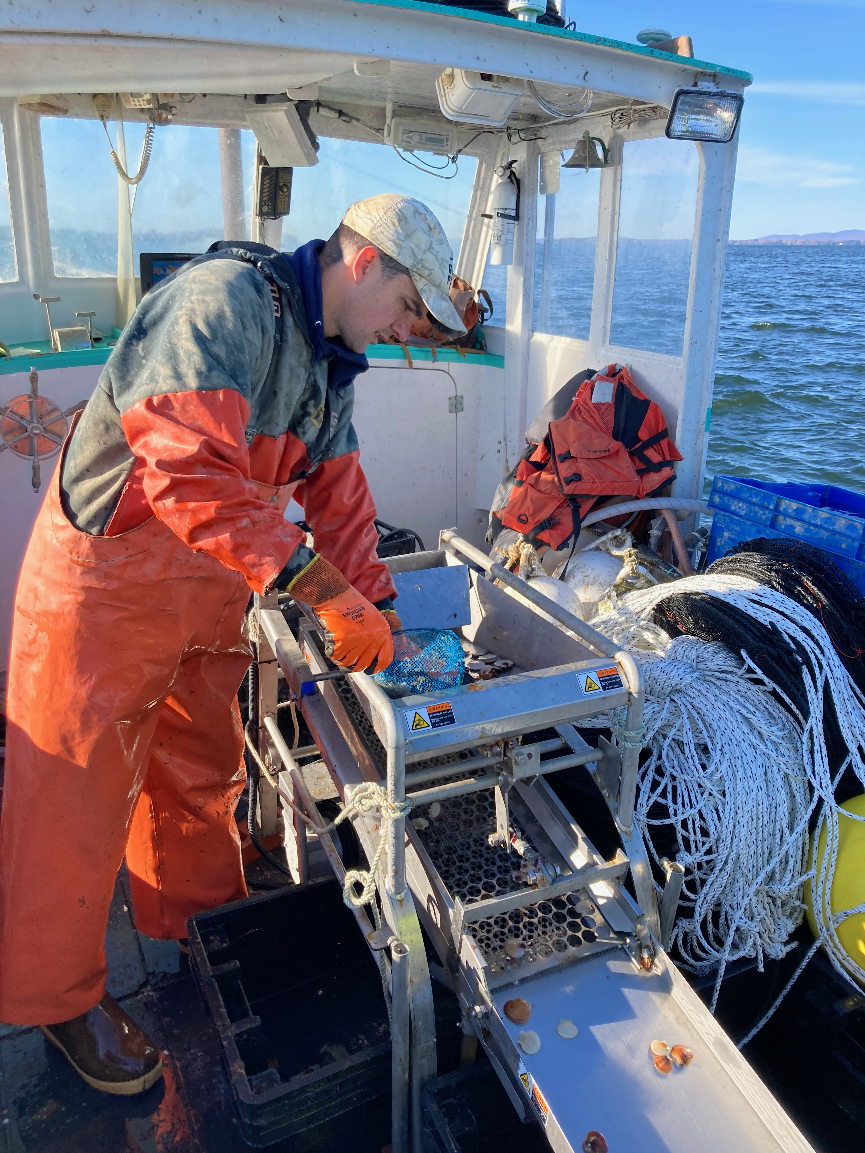 We sourced the specialized scallop grader from Japan to grade scallops into distinct size classes. We also trialed the same model scallop grader (see photo and video), courtesy of Coastal Enterprises Inc., on Andrew Peter's vessel (the partner farmer). Preliminary grading sessions indicated that the equipment is compatible with all electrical sources on Andrew's vessel and is (albeit anecdotally) effective at sorting farmed scallops into various size classes. We are continuing to monitor the growth of the scallops that will be used in the upcoming ear-hanging season and await the arrival of Andrew's grader.
Click here to watch video clip of the scallop grader.
2022
June: "early" ear-hanging date
We initiated the field portion of the project on June 7th, 2022. Andrew Peters hosted a team of researchers from the University of Maine on his vessel to (1) trial the scallop grader ordered from Japan, (2) sort juvenile scallops from lantern nets and run the cohort through the grader into distinct size classes, (3) ear-hang sorted scallops, and (4) measure the initial size of the ear-hung scallops for the growth and mortality trials. We emptied 12 lantern nets and graded ~2 thousand scallops over the course of the morning into small, medium, and large cohorts, which corresponded with grade size of <=53 mm, between 54 and 60 mm, and >61 mm, respectively. We then ear-hung all graded scallops, keeping like size grades together on individual dropper lines. Please see the video below for a demonstration of ear-hanging (i.e., drilling and pinning scallops).
We took initial scallop shell height measurements (the distance between the dorsal hinge and the furthest point of the ventral edge of the shell) of scallops on 6 dropper lines: 3 lines from the "Small" grade (scallops <=53 mm) and 3 lines of the "Large" grade (scallops >61 mm). We measured the top 40 scallops on each line, for a total of 240 measurements, to the nearest mm using calipers. This measurement date represented our "Early" ear-hanging deployment.
August: "Late" ear-hanging date
On August 11th, 2022, Andrew Peters hosted the same group of UMaine researchers on his vessel out of Belfast Harbor, ME. We measured the top 40 scallops from each of the 6 dropper lines that were ear-hung on the "early" deployment date (June 7th) to record changes in shell height. Each line was assessed for mortality as well.
Due to the extreme heat on the sampling day, our industry partner, Andrew Peters, decided to not use the scallop grader to sort a new cohort into like sizes. Rather, a new batch of scallops was emptied from 20 lantern nets and ear-hung (without grading) using the same drilling and pinning methods as those from the June measurement date. These scallops represent our "Late" ear-hanging treatment. Initial shell height measurements were recorded for the top 40 scallops on each of 6 six lines chosen haphazardly for the experiment.
The fact that it was too warm to grade on the August date is a useful data point as we begin to solve the grading and ear-hanging puzzle. If ambient air conditions are not suitable for grading and ear-hanging in the late summer, ear-hanging early may have advantages with respect to survival and scallop performance in the weeks following grading, drilling, and pinning.
November: growth and mortality assessment between treatments
On November 6th, 2022, all 12 experimental dropper lines were measured for changes in shell height and mortality. The same sampling protocol was carried out: the shell heights of the top 40 scallops on each line were recorded to the nearest mm using a caliper.
We plan to visit the site again in March (the start of the scallop harvest season) to record final changes in shell height between the "early" and "late" ear-hanging treatments, assess meat yield for market, and gather final info for our economic analysis of grading and ear-hanging scallops in Maine.
Video 1, depicts Andrew Peters, founder and CEO of Vertical Bay Maine (our partner farmer) drilling scallops in preparation for ear-hanging.
Video 2 depicts ear-hanging "dropper" lines tied to the horizontal longline after the ear-hanging process on Vertical Bay's lease in Penobscot Bay
March: final measurement
On March 11th, 2023, we completed the final assessment of shell height growth, mortality, and meat weight (adductor muscle) at the site.
Study results
Biological growth and mortality data.
On June 7 2022, we graded scallops into Small and Large cohorts using the automated scallop grader imported from Japan. The equipment performed well. We were able to produce two distinct size classes prior to ear-hanging in a relatively efficient manner that can be improved over time (2,000 scallops graded in ~30 minutes). After grading, the scallops in the large cohort ranged from 50 - 70mm, despite the fact that a screen with 60mm diameter holes was used. This indicates that the grader may not produce incredibly accurate size grades and should be taken into consideration when trying to optimize the equipment. The scallops in the Small grade (screened using <53 mm holes) were between 30 - 60mm (Figure 1). The scallops that came out of nets and were ear-hung in August were ungraded, and ranged from 50 - 70 mm (Figure 1).
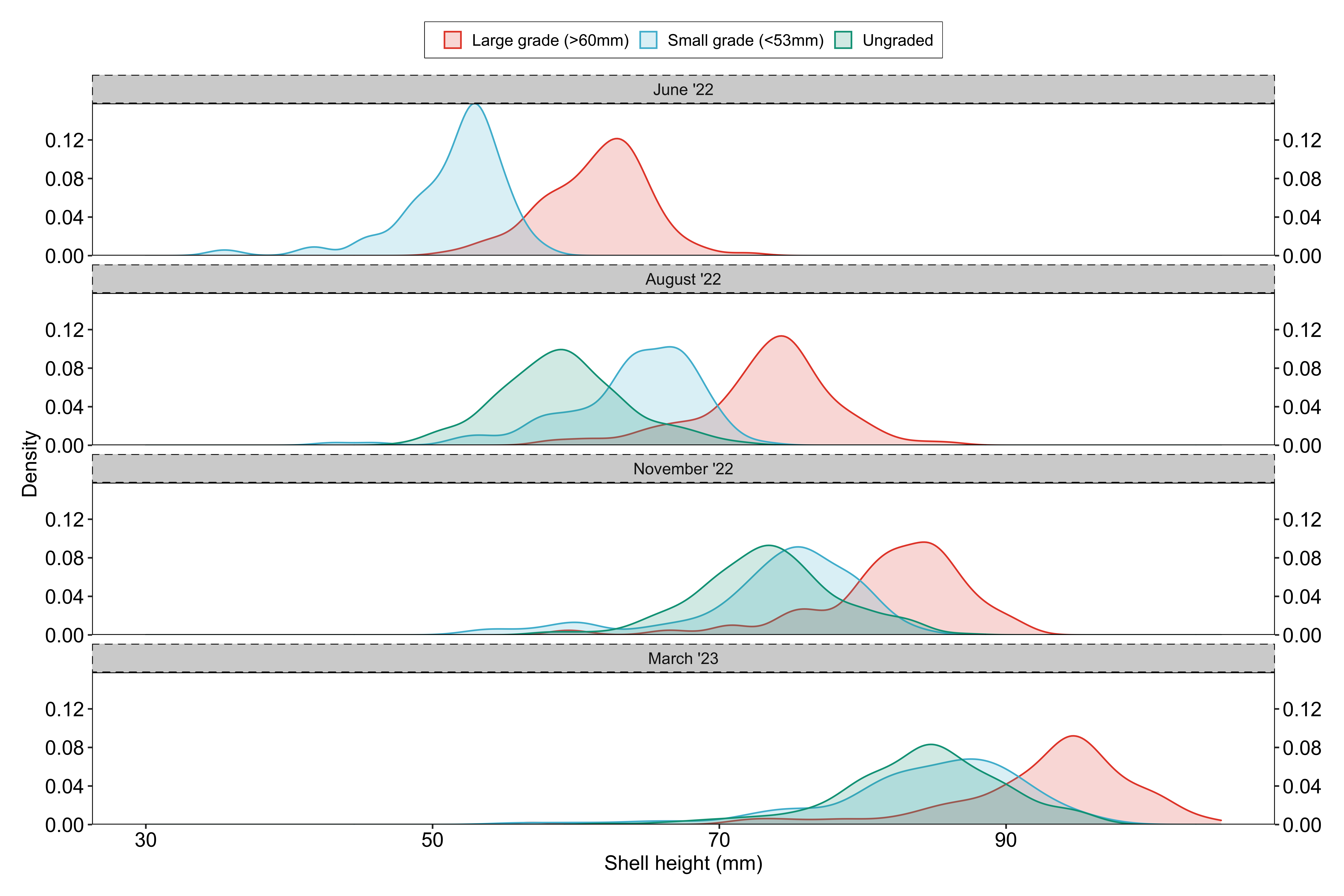
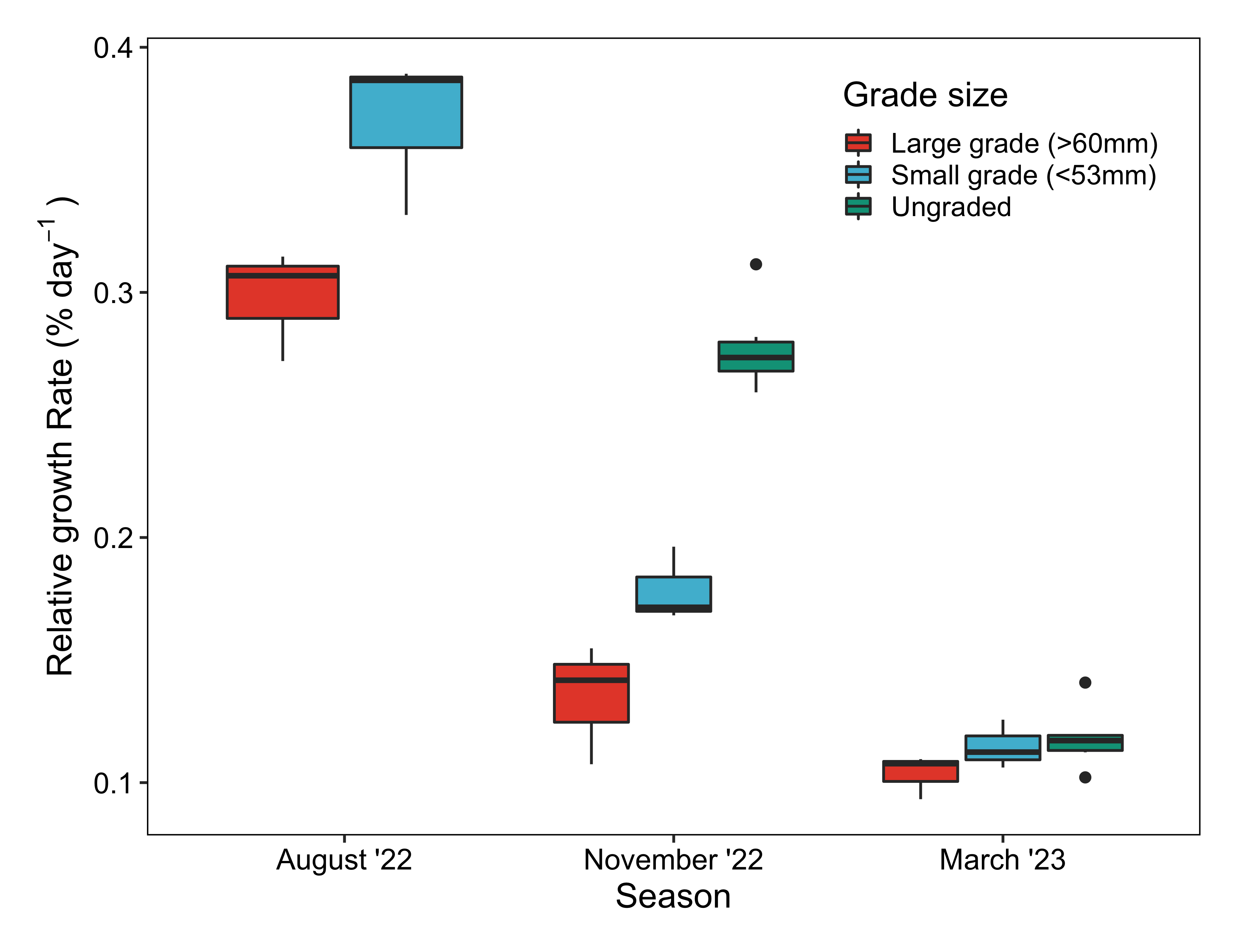
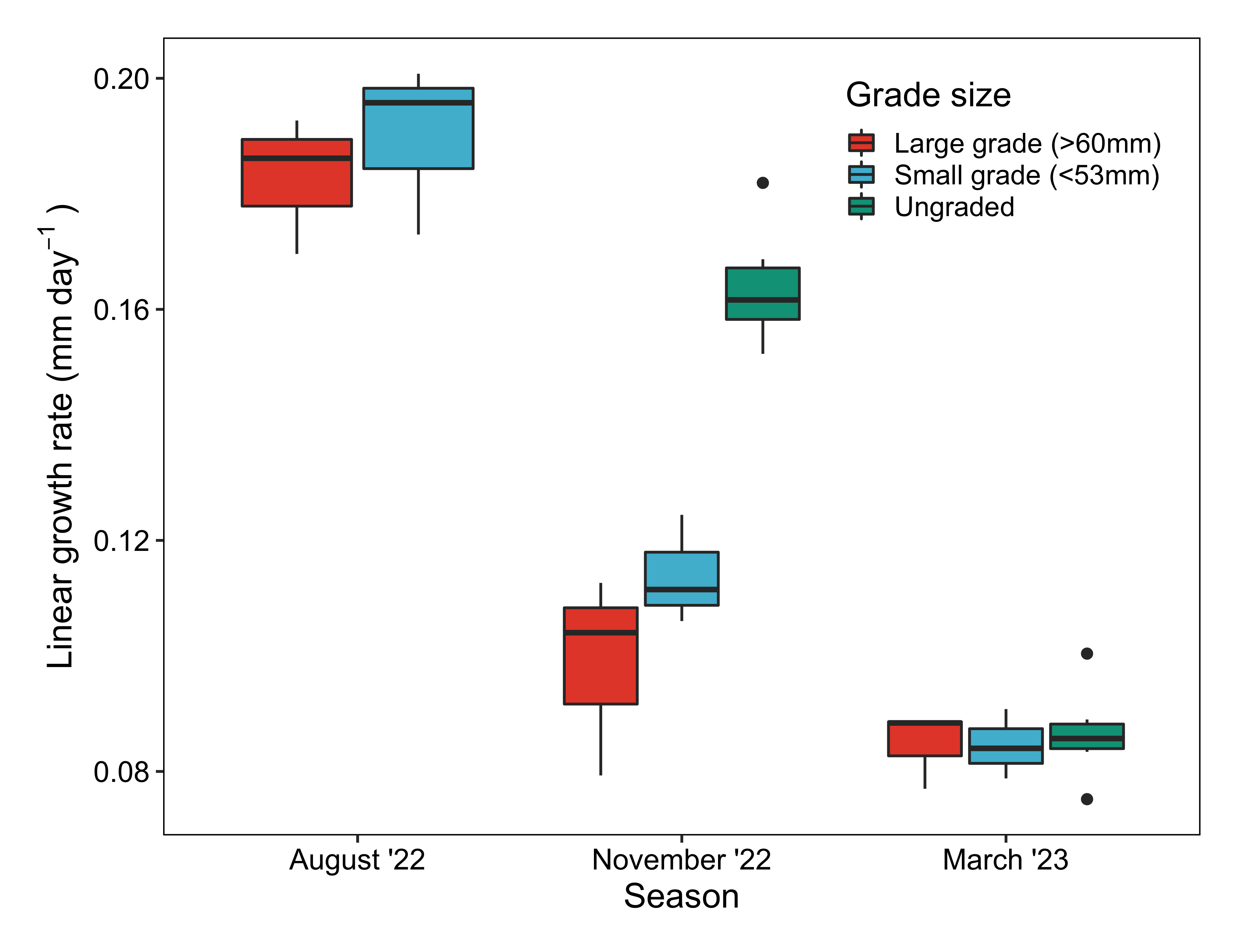
Over the course of the 10-month study period, the scallops in the large cohort grew from an average of 61.4 mm to an average of 92.5 mm, and average growth rate of 0.12 mm / day and 0.18% / day (Figure 2a, 2b). Interestingly, the scallops in the ungraded, "late" ear-hung cohort grew very similarly to those in the early ear-hung, small cohort, displaying very similar shell height distributions in March 2023 (Figure 1).
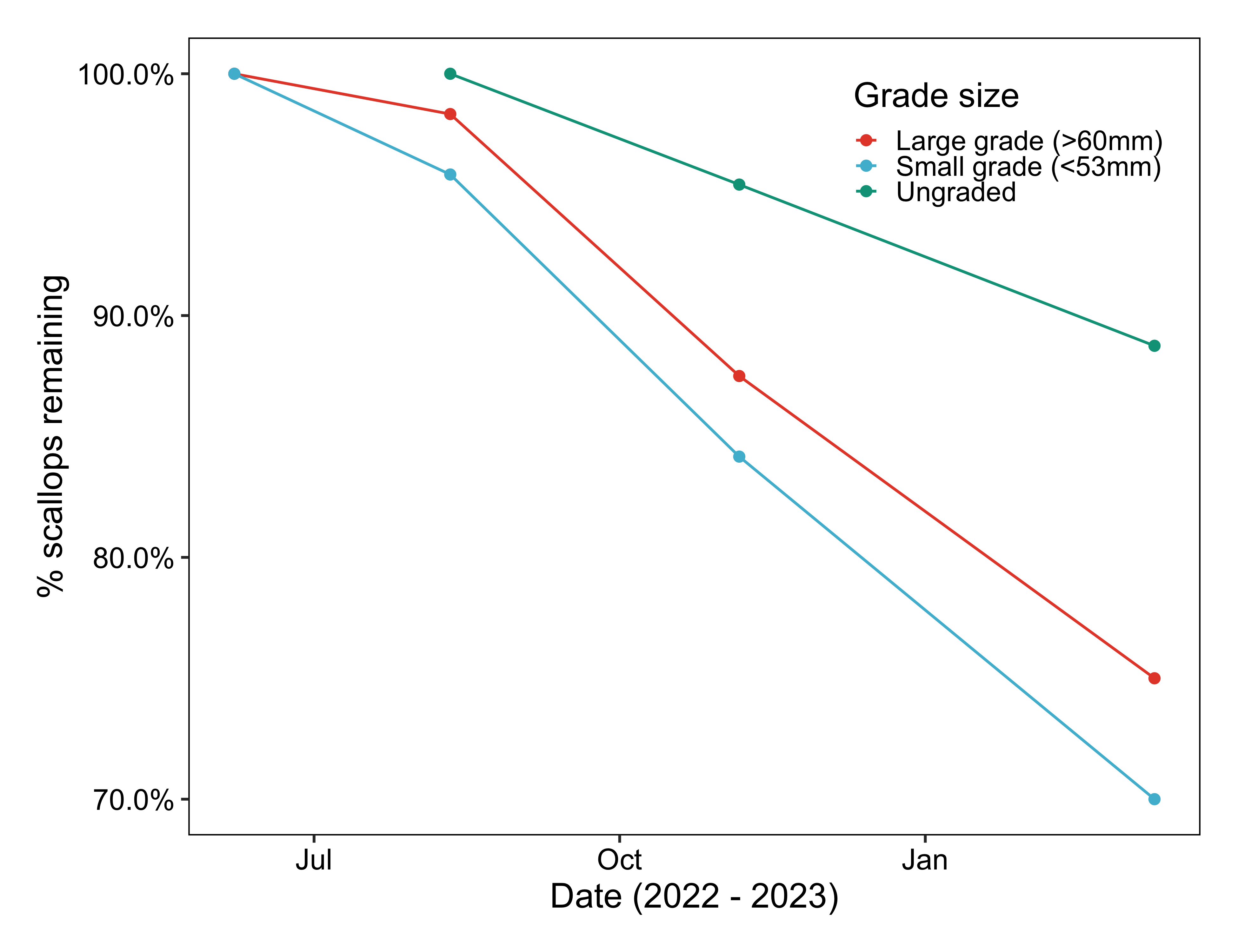
The mortality rate over the course of the study was highest for the scallops in the "Early" ear-hung, small grade cohort, and lowest for the ungraded, "late" ear-hung scallops. At the end of the study, only 70% of the June ear-hung, small grade scallops remained alive on the dropper lines, while nearly 89% of the ungraded, August ear-hung scallops remained (Figure 3).
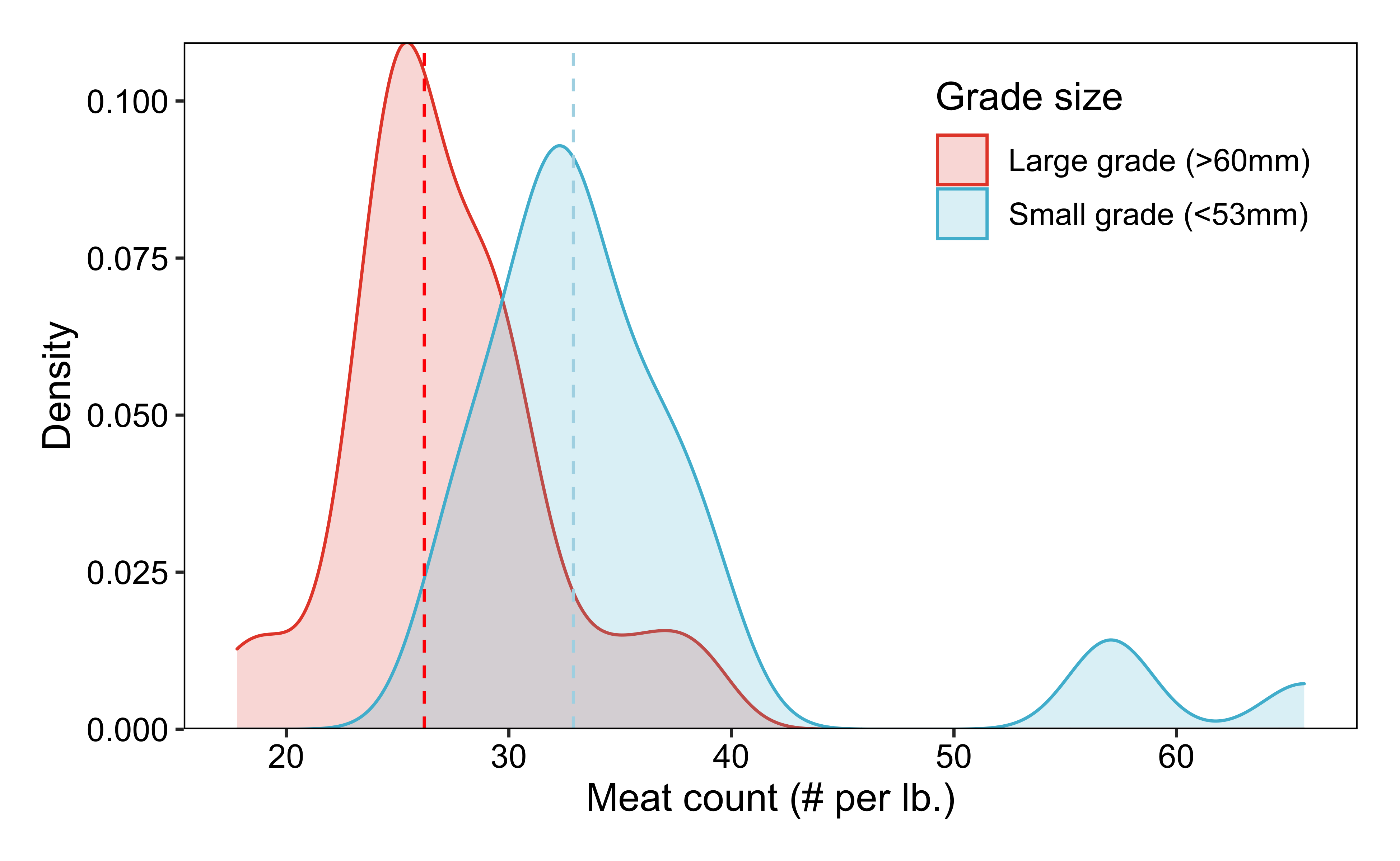
At the end of the study in March 2023, the scallops in the Large and Small, early ear-hung cohorts had average meat sizes of 17.1 and 13.3 g, which corresponds to meat counts (# of scallops per lb.) of 26.5 and 34.1, respectively. Based on the distribution of the meat sizes within the two cohorts, the Large grade had many more scallops in 30 - 40 count range, while the Small grade was centered more around a 25 count meat (Figure 4).
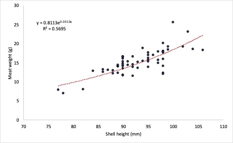
Using the meat weight data, we derived a relationship between shell height and meat weight that we then applied to all of the final shell height measurements on the final sampling date (March 2023). We fit an exponential regression to the pooled Large and Small cohort data (R2= 0.57) and then used the best fitting equation to predict the meat weight of the 420 data points collected on the same date (Figure 5).
Bioeconomic model results
Based on the growth and mortality data collected over the course of the study, and leveraging the experience of our partner farmer Andrew Peters, we were able to parameterize a simple bioeconomic model of ear-hanging to explore the financial implications of ear-hanging "Early" vs "Late" in the season. The cost inputs were identical between the two simulations. In both cases, we constructed a hypothetical farm that was starting with 500,000 scallops in June and ear-hanging in either June or August. We then quantified total biomass, and the value of the biomass based on the relative proportions of scallops within specific size classes, to estimate the potential tradeoffs between the two strategies.
Based on the growth and mortality data, the "Late" ear-hanging method produced more biomass (lbs. of scallops) at the end of the season. Despite lower overall growth rates, the higher survival rate within the ungraded, late ear-hanging cohort outweighed any growth disadvantages that this strategy may produce. This resulted in a lower overall production cost ($ per lb. produced) and higher theoretical profit margin for the "Late" ear-hanging simulation (Table 4).
| Table 4. Summary bioeconomic model outputs | "Early" ear-hanging (June) | "Late" ear-hanging (August) |
| Inventory | ||
| Scallops | ||
| % Q1 | 58,906 | 122,031 |
| % Q2 | 52,865 | 147,917 |
| % Q3 | 95,156 | 127,578 |
| % Q4 | 155,573 | 46,224 |
| Total (inds.) | 362,500 | 443,750 |
| Biomass | ||
| Q1 (lbs.) | 1,160 | 2,403 |
| Q2 (lbs.) | 1,301 | 3,639 |
| Q3 (lbs.) | 2,683 | 3,597 |
| Q4 (lbs.) | 5,454 | 1,621 |
| Total (lbs.) | 10,598 | 11,260 |
| Value of inventory | ||
| Q1 ($) | $17,776 | $36,826 |
| Q2 ($) | $20,546 | $57,488 |
| Q3 ($) | $43,699 | $58,588 |
| Q4 ($) | $91,580 | $27,210 |
| Total ($) | $173,601 | $180,112 |
| Cost of goods | ||
| Labor | $28,286 | $28,286 |
| Fuel | $7,071 | $7,071 |
| General consumables | $186 | $186 |
| Pins | $3,750 | $3,750 |
| Total COGS | $39,293 | $39,293 |
| Gross profit | $134,308 | $140,819 |
| Overhead | ||
| Depreciation | $11,582 | $11,582 |
| Lease rent ($100 / acre / year) | $1,429 | $1,429 |
| Insurance and other overhead ($100 / acre / year) | $1,190 | $1,190 |
| Total overhead | $14,201 | $14,201 |
| Net margin | $120,107 | $126,618 |
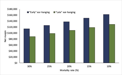
However the results were sensitive to changes in the mortality rate associated with each pathway. The figure below shows the results of the same simulation, but at consistent levels of mortality between the early and late simulations. If the mortality is the same between the two methods, the higher proportion of larger, high value scallops in the "early" ear-hanging treatment provides an economic advantage (Figure 6).
Over the course of the experiment, we identified some concrete methods to improve the scalability and feasibility of scallop aquaculture by making adjustments to the schedule of ear-hanging. We set out to measure the feasibility of (1) using the custom fabricated scallop grader to sort inventory into discrete size classes prior to ear-hangin, (2) quantify the impacts of size grading and the timing of ear-hanging (either "Early" or "Late") on growth and mortality, and (3) integrate the scallop growth data within a simple economic model of scallop farming to project the potential financial implications of adjusting the timing of ear-hanging.
We observed that scallops ear-hung in June ended up larger than the same seed cohort that was ear-hung later in the season in August. However, we also noted that scallops that were ear-hung in June saw increased mortality levels when compared to the August ear-hanging treatment. We suspect that this was not a product of size. When we looked at all scallops graded in June, the difference in the mortality rates between the "Large" and "Small" grades was far less pronounced than the difference in the mortality rates between the "Large" size class ear-hung in June and the "Ungraded" scallops ear-hung in August. We suspect that mortality is simply higher on dropper lines that in lantern nets. This should be an active area of focus and R&D for the industry.
Our results suggested that ear-hanging earlier in the season may be an effective strategy of improving the economics of an individual farm. If farmers are able to fetch a premium for larger meats, even under elevated mortality levels ear-hanging earlier may be beneficial. However, controlling mortality should be a top priority for growers. There are likely unexpected benefits and challenges to ear-hanging earlier in the season. This work provides a critical first step in optimizing the timing of the process and expanding scallop farming in Maine.
Education & outreach activities and participation summary
Participation summary:
The ability to effectively communicate the results of this work to industry, public, and research audiences is one of the strong suits of the project team. Coleman is adapting a bioeconomic model of scallop lantern net aquaculture to be used as a budgeting tool with aquaculture business specialists at the Maine Aquaculture Association (MAA). MAA is a non-profit trade association that represents Maine Aquaculturists and provides business planning tools for both new and experienced growers. Despite the fact that interest in scallop aquaculture is rapidly growing in the Northeast U.S., little information exists to help growers project future profits and losses based on current production practices. The financial models generated from this project would not only be used as an analytical tool by the UMaine research team, but also incorporated into MAA's suite of business planning tools for new and experienced growers.
Brady is a contributor to the Aquaculture in Shared Waters (ASW) class, a hands-on technical workshop run annually by University of Maine Sea Grant. ASW annually prepares ~ 75 fishermen and farmers to operate aquaculture businesses, exposing them to a diversity of species (seaweed, oysters, mussels, and scallops), and culture methods. The technical and financial information from this project would be readily incorporated into the ASW scallop unit, as little information currently exists regarding the efficacy of ear-hanging from a business standpoint.
Mr. Peters is a member of the Maine Aquaculture Co-op (MAC). Coleman also attends MAC meetings and contributes scientific and research updates. The MAC hosts the majority of scallop growers in Maine. Mr. Peters and Coleman will relay the results of this information back to MAC growers. MAC members, other than Mr. Peters, have also made substantial investments in ear-hanging equipment, and the results of this study would be directly applicable to their businesses.
Lastly, Brady and Coleman plan to publish the results of the ear-hanging bioeconomic analysis in a relevant academic journal. As mentioned above, the UMaine research team has experience formally analyzing scallop growth and mortality data and building aquaculture financial models. This work will fill a data gap that would be readily useful to managers, industry, and the academic community.
To date, we have conducted 3 field days and 2 farm equipment demonstrations with other scallop growers. Using the same model scallop grader that we have ordered for the project, on a short term loan from Coastal Enterprises Inc., we have conducted a "dry-run" of scallop grading with juvenile "seed". As a result of this connection, we have also coordinated with Coastal Enterprises Inc. (CEI) on the purchase of the grader. We have received the new scallop grader from Japan and have begun trialing the equipment on Andrew Peter's boat. This machine, as a result of SARE support, will be utilized in the upcoming season to improve ear-hanging efficiency and make the following year's harvest much more streamlined as like sized scallops will be kept together.
Learning Outcomes
As a result of the first field day and grader demonstration (see photos attached), we shared knowledge related to the specialized equipment with one other scallop farmer. We have since visited the farm multiple times to record project data and have shared our work plan and very preliminary findings with other growers, researchers, and extension agents.
We hope to make concrete recommendations regarding the optimization of ear-hanging once we have made our final site visit in March, analyzed the growth data, and built our financial model of scallop farming. We anticipate that this information will help farmers make more informed decisions and improve the sustainability of scallop aquaculture in Maine.
After our final visit in March, we were able to analyze the data (both biological and production oriented) to make decisions regarding best practices and potential cost reduction strategies. We hope to continue to investigate the "Early" ear-hanging strategy as a scalable farming method.
Project Outcomes
The project began in June, 2022. Since that date, we have made 3 field visits to record operational and scallop biological data, shared findings with other research and industry members, and begun to analyze very preliminary scallop growth and farm economics data. We plan to share our findings with not only our industry partner, Andrew Peters of Vertical Bay, but also other interested scallop farmers in Maine, researchers, regulators, and the public.
We view scallop farming as an incredibly powerful income diversification tool for the state of Maine. Optimizing the economic performance of farms using automated equipment can improve farm owner/operator livelihoods. We plan to make our final measurement and analyze all project data (biological and economic) in March.