Final report for SW18-103
Project Information
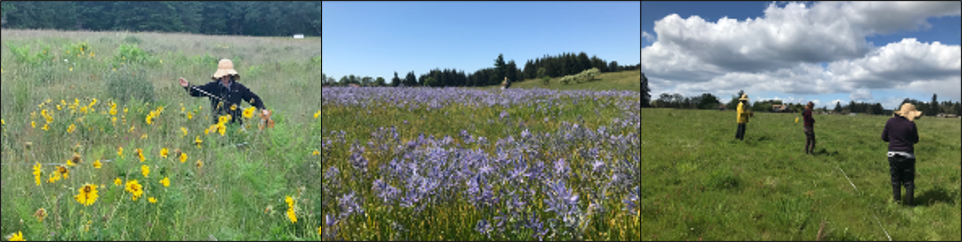
Most rangelands west of the Cascades in the Pacific Northwest occur on sites that historically supported native prairie. Over 90% of the prairies in this region have been converted to agriculture or lost to development, making conservation of this rare system a top conservation priority. At the same time, the human population in this region continues to grow, demanding more from regional food production systems. Therefore, agricultural producers are under great pressure from growing needs for food production and habitat conservation. Because of this, it is increasingly recognized that effective prairie conservation can only be achieved by partnering with private landowners to develop incentivized conservation strategies that maintain productive farms. Through a unique collaboration between agricultural producers, conservation scientists, economists, sociologists, regulators and agricultural researchers, we propose to evaluate if and how agricultural productivity can be maintained or enhanced in working landscapes while simultaneously accruing conservation value for rare native plants and animals. Through replicated on-farm experimental demonstrations, we will quantify the ‘ecological lift’ generated by conservation tools (altered grazing regimes, spring rest period, seeding native species). Additionally, we will evaluate the costs and benefits associated with conservation actions, to provide guidance on strategies and expenses for agricultural producers. Finally, we will survey producers to identify concerns, questions and needs (financial, technical, other) surrounding habitat conservation on their properties. The combined ecological, economic and social survey data will help guide government incentive programs. We expect this work to identify opportunities for agricultural producers to increase the conservation value of their properties, while maintaining or even enhancing their bottom line. Study findings and educational materials resulting from the demonstration trials will be communicated through peer-reviewed publications, presentations at academic conferences, a published grazing management guidebook, and a series of collaborative regional workshops for agricultural producers, researchers, extension agents, and land managers.
- Develop a regional network of three grazed prairie research sites to demonstrate and evaluate effects of conservation tools on prairie habitat. This objective will:
- Implement conservation tools for target species and habitats, with focus on management intensive grazing, exclusion during critical flowering periods and/or native seeding.
- Evaluate impact of conservation installations through a range of habitat and species abundance metrics over 3 years.
- Utilizing the regional network of grazed and ungrazed prairie sites, quantify the financial benefits and costs associated with managing critical habitat and species on grazed prairie as compared to ungrazed conservation prairie over a 3-year period. This objective will:
- Provide practical financial information to farmers, the conservation community, and the county planners concerning the costs of meeting HCP requirements on grazed and ungrazed prairie both on private and protected sites.
- Develop enterprise budgets and a benefit-cost analysis to inform HCP acreage targets for protecting critical species on grazed land relative to conservation preserve land.
- Engage private landowners by administering a social survey focused on landowner needs for increased involvement in land conservation programs (conservation easements, HCP, Safe Harbor Agreement). This objective will:
- Engage producers and regulatory entities in a productive discussion on incentives needed for habitat conservation on working lands.
- Provide feedback for regulatory programs on effective strategies to engage private landowners.
- Present opportunities for technical assistance related to habitat management and discuss economic and landowner incentive opportunities with agricultural producers, regulatory agencies and conservation land managers through several mechanisms:
- Workshop series, with field tours of the agricultural demonstration sites and native prairie preserve sites. Field tours will be sponsored by WSU, CNLM, Thurston County Conservation District and NRCS.
- WSU-Extension technical bulletin providing management guidelines and financial data for conservation tools; and two published manuscripts in peer-reviewed journals.
- Presentation of findings at regional and national conferences.
Cooperators
- - Producer (Researcher)
- - Producer
- - Producer (Researcher)
Research
- Implementation of conservation grazing practices will shift habitat value towards that of ungrazed native upland prairie, as measured by native species richness, percent native groundcover, and butterfly behavior.
- Occupancy of endangered or threatened species, such as Mazama pocket gopher, is not significantly different between grazed and ungrazed prairie sites.
- Implementation of conservation grazing practices will not reduce overall forage productivity.
- Integrating conservation practices into grazed working lands will not disrupt the economic cost:benefit balance for the farmer.
- Integrating grazed working lands into conservation practices can result in significant economic contributions to the regional economy
- Appropriate and beneficial incentives and approaches can be identified from farmers and ranchers to improve participation and trust in conservation programs and conservation partners.
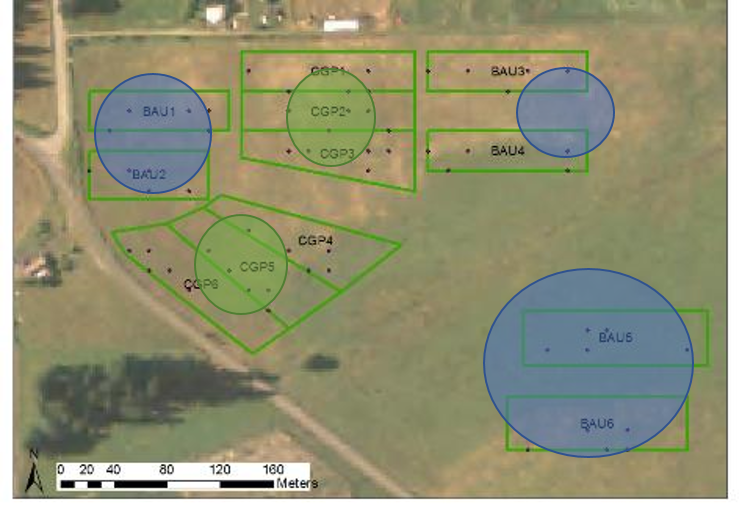
Three farm sites (Colvin Ranch, Fisher Ranch and Riverbend Farm) and three ungrazed prairie sites (Johnson Prairie, West Rocky Prairie, and Wolf Haven) were chosen for this study to represent a range of forage quality and practices and upland prairie habitat conditions. Within each farm site, six 1-acre paddocks were chosen for Conservation Grazing Practice (CGP) treatments (n=30), along with paired 1-acre Business as Usual (BAU) paddocks (n=30) (see site maps in Appendix A). Assigned CGP treatments were developed through the NRCS Site Inventory Planning process (NRCS, 2017) and reflect site-specific conditions and desired natural resource outcomes for each ranch (Table 1).
Table 1. Business as Usual and Conservation Grazing Practice Treatments for each farm site
|
Farm Site |
BAU Treatment |
CGP Treatment |
|
Colvin Ranch |
MiG with spring deferment |
Native seeding |
|
Fisher Ranch |
Rotational grazing w/ spring deferment |
Rotational grazing w/ spring deferment and native seeding |
|
Riverbend Farm |
Continuous grazing |
Rotational grazing w/ spring deferment and native seeding |
Six areas within each of the selected native upland prairie (NUP) sites were also chosen as replicate plots to provide a comparison to the BAU and CGP treatments at the farm sites (Appendix A). We placed a 15 m x 15 m grid over maps of each of the 1-acre treatment plots at each site and randomly chose 5 subplots within each treatment plot. A range of community and species-specific variables were measured in these plots (Table 2).
Table 2. Parameters measured
|
Treatments (independent variables) |
Business as Usual grazing (BAU), Conservation Grazing Practices (CGP), Native Ungrazed Prairie (NUP) |
|
Site responses (response variables in BAU and CGP) |
Forage residue (biomass) in 2018 with additional measures planned for 2019-20: forage quality (ADF, NDF, CP, TDN) |
|
Plant community (response variables) |
Native and non-native species richness and diversity, percent cover of trees, shrubs, forbs, native grass, and forage grass; abundance of butterfly nectar and host plants |
|
Gophers (response variables) |
Gopher mounds/grid cell |
|
Butterfly behavior (response variable) |
Move lengths, turning angles and diffusion rates |
|
Soil measures (response variable |
Soil temperature, soil bulk density |
|
Soil measures (site-level co-variates) |
Soil classification, soil nutrients |
Vegetation monitoring
To determine the native and non-native species richness in each site and each treatment, we recorded all plant species present in each of the five 15 m x 15 m subplots within each plot in each treatment (CGP, BAU, NUP) in May-June 2018-2020. Additionally, we recorded the percent cover of trees, woody shrubs, native forbs, forage species, native grasses, and abundance of butterfly resource species in each subplot (Figure 2). Finally, we measured the abundance of seeded species in four 1 m x 1 m quadrats in each subplot.

To evaluate changes in plant community composition, we used Non-metric Multidimensional Scaling (NMDS) and mixed effects models (i.e., Generalized Linear Mixed Models (GLMMs) and standard linear mixed models). We excluded native ungrazed prairies from our analysis to simplify the models and focus on differences between the CGP and BAU treatments. For each response variable, we applied the mixed model that best fit the data distribution (i.e., native species richness = quasi-Poisson GLMM, non-native species richness = Gaussian linear mixed model, and native forb cover = beta GLMM in conjunction with a hurdle model to account for zeros). Year, treatment, and site were modeled as fixed effects while sampling plot was nested within paddock (both considered random effects). Additionally, our models were structured to account for repeated sampling of the same plots each year. After running each model, we performed an Analysis of Deviance (Type II Wald Chi-square test) to determine the significance of each fixed factor and the year*treatment interaction. Significant results were examined by pairwise comparisons with Bonferroni corrections to elucidate differences within factors (e.g., differences between sites or between years) and to tease apart year*treatment interactions.
Gopher monitoring
Mazama pocket gophers are 100% fossorial, making measures of abundance extremely difficult and labor intensive. Instead of tracking abundance through live-trapping, we have chosen to track presence/absence sign (i.e., mounds; Figure 3) and use these data to determine occupancy estimates. Occupancy as a metric of population status that indicates the proportion of the landscape that is being utilized by the target species. This technique requires repeat visit surveys of fresh mounds (< 48 hrs. old) within the treatment areas so that seasonal and annual impacts to mound-building are accounted for. We visited plots three times in Fall 2018, 2019 and 2020 with a 3- to 4-day interval between visits. Each survey consisted of searching plots for two minutes or until fresh gopher mounds were located.
Forage cover of preferred and less preferred species
While vegetation monitoring occurred at all sites, a targeted sub-analysis of forage cover was completed at one participating ranch that implemented a paddock conservation grazing system alongside business as usual grazing for this study. This site, Riverbend Ranch, afforded an opportunity to evaluate the effect of planned grazing on forage cover, particularly on the balance of perennial and annual forage species, and more- or less-preferred grass species.
Percent cover of forage species was estimated by applying a point-intercept method using a cross-hair point frame. A 1m x 1m PVC frame was constructed with four strings arranged in a grid at equidistant intervals resulting in a total of 16 intercept points. Each of the six total replications at the ranch site was sub-sampled four times. The sampling frame was placed 1 m to the northwest of the inside southwest corner of the 15m x 15m subplots established for vegetation monitoring described above. Six subsample quadrats per replication were developed for the native vegetation surveys. Subplot corners were geo-located using Avenza.
A data sheet was developed to record every grass or forb species that intersected a metal pin flag placed successively at each grid intersect on the cross-hair frame. Field data collection occurred on June 4th, 2021. Following field data collection, total counts were obtained of all grasses, forbs, perennials, annuals, biennials, and more preferred and less preferred grass species. Table 3 identifies assumptions regarding more/less preferred species. Identification of preferred grass species were based species lists and rankings in the Washington State University Extension Bulletin Pasture and Hayland Renovation for Western Washington and Oregon (Fransen and Chaney 2014). To be considered “more preferred”, species were ranked at a minimum moderate for both palatability and yield, and rated ‘high’ for at least one of these two parameters.
Table 3. “More preferred” and “less preferred” grass species as defined for the forage cover analysis
| More preferred grass species | Less preferred grass species |
|
Festuca arundinacea Festuca roemeri Dactylis glomerata Poa pratensis |
Bromus hordaceous Agrostis capillaris Vulpia bromoides Anthoxanthum oderatum Cynosaurus cristatus Poa annua Holcus lanatum |
Gopher monitoring
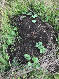
Mazama pocket gophers are 100% fossorial, making measures of abundance extremely difficult and labor intensive. Instead of tracking abundance through live-trapping, we tracked presence/absence of mounds (Figure 3) and use these data to determine occupancy estimates. Occupancy is a metric of population status that indicates the proportion of the landscape that is being utilized by the target species. This technique requires repeat visit surveys of fresh mounds (< 48 hrs. old) within the treatment areas so that seasonal and annual impacts to mound-building are accounted for. We visited plots three times in Fall 2018, 2019 and 2020 with a 3- to 4-day interval between visits. Each survey consisted of searching plots for two minutes or until fresh gopher mounds were located. To understand how our experimental factors influenced gopher occupancy, we ran a binomial GLMM and post-hoc analyses similar to those we ran for the vegetation data. However, we included native ungrazed prairies in the analyses to compare gopher occupancy across ranches and native prairie sites
Butterfly behavior
While some grazing may have beneficial impacts on prairie plant communities, other taxa may have unique responses to grazing pressure (van Klink et al 2015). Lepidopterans, particularly butterflies, make good indicator species for the effects of grazing because they are sensitive to changes in their environment since they use very different parts of the ecosystem in adult and larval stages (Kerr 2000). Prominent studies on the effects of grazing on grassland butterflies in Europe have found positive effects of low-intensity, extensive grazing by maintaining plant community diversity, lowering vegetation height, and creating heterogeneity on a pasture and regional scale (Bussan 2022, Pöyry et al 2004, WallisDeVries et al 2016, Jerrentrup et al 2014; but see Kruess and Tscharnske 2002). There is comparatively little research on butterfly responses to grazing in North America, often with more mixed results (Bussan 2022, Weiss 1999, Delaney et al 2016, Debinski et al 2011).
We use butterfly behavior and movement as a proxy for habitat quality. Animals change their behavior when encountering changes in their environment. Animals will exhibit “area restricted search” when encountering high quality (resource-rich) habitat, meaning that they will take shorter steps between turns and larger turning angles (Kareiva and Odell 1987, Turchin 1998). This will effectively slow their rate of movement through their habitat. Many studies have used this behavior to describe some aspect of habitat, land cover, or resources animals are encountering (e.g. Stevens et al 2004, Brown et al 2017). By quantifying an animal’s rate of movement (i.e. its diffusion rate) through its habitat, we can classify perceived habitat quality (Schultz et al 2019). In addition, we can compare butterfly behavior and movement as a measure of butterfly preference, and vital rates (survival and fecundity) as a measure of butterfly performance. Together preference and performance are measures of the effective habitat quality, i.e. whether a habitat is a potential demographic source or demographic sink (Pulliam 1988).
We conducted two different experiments using two common native butterfly species. In the first experiment, we compared butterfly behavior and diffusion rates in grazed pastures and in native prairie to determine factors that influence their movement through both environments and obtain an index of habitat quality based on butterfly habitat perception. The second experiment was a modified preference-performance study (Thompson and Pellmyr 1991) to test whether there was a difference between the BAU and CGP on Riverbend Ranch treatments in terms of larval survival (“performance”) and adult edge behavior (“preference”), and if so, whether the adults preferred the treatment that maximized larval performance.
Butterfly behavior/movement questions and hypotheses
Question 1: How does cattle grazing management influence butterfly movement rates and habitat perception? Hypothesis 1: Using diffusion rate as an index of movement behavior, butterfly diffusion rates will be highest in “conventional” grazing, intermediate in “conservation” grazing, and lowest in native upland prairie.
Question 2: How do nectar and host plant resources and vegetation structure influence butterfly behavioral response to habitat? Hypothesis 2: Butterfly diffusion rates will differ depending on the resources available to them along their flight paths. Diffusion rates will be lower when nectar and host plant resources are high and diffusion rates will be higher when nectar and host plant resources are low.
Butterfly preference/performance questions and hypotheses
Question 3: How does grazing management influence butterfly preference and performance? Hypothesis 3: Butterflies will show greater preference and higher performance in CGP paddocks.
General butterfly study methods
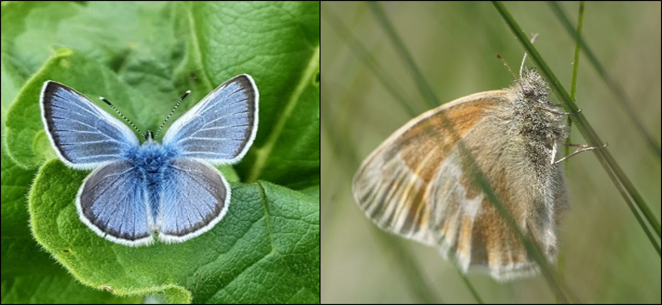
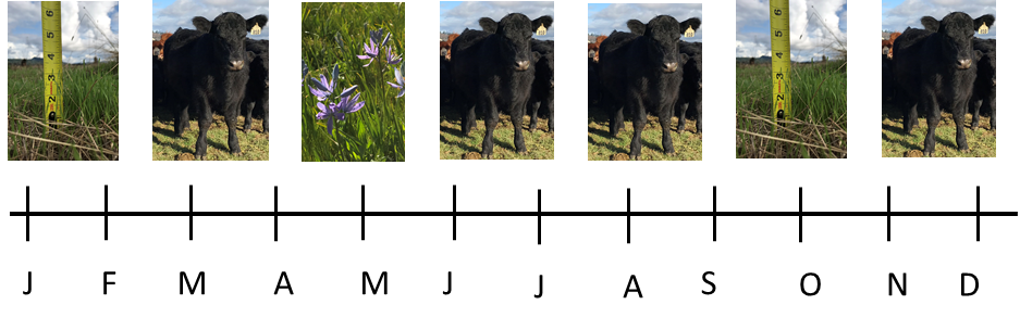
In all years, we observed two common native butterfly species, which allowed us to account for differing habitat needs and phenology (Figure 4). The first species, silvery blue butterfly (Glaucopysche lygdamus), is distributed throughout the western US and is hosted by lupines and vetches. The adults fly from the end of April to the end of May/early June in Western Washington prairies. The second species, ochre ringlet (Coenonympha california) is also distributed throughout the western US, but the subspecies we are working with (C.c. eunomia) is concentrated mainly in the South Puget Sound. Ochre ringlets are hosted by various grass species and are bivoltine. The adults fly from early May to mid-July and from late July to early September.
We chose nine sites in western Washington (Table 1). Seven are part of the South Puget Sound prairie ecosystem in Thurston County and are part of the main grazing experiment described elsewhere in this report (Colvin Ranch, Riverbend Ranch, Fisher Farms, Johnson Prairie, West Rocky Prairie, and Wolf Haven Prairie). Two are part of the Boistfort prairie ecosystem in Lewis County (Maynard and Mary Mallonee’s farms). Six are grazed as part of active cattle and dairy farm operations. Of the grazed sites, three (Colvin Ranch, Fisher Farms, and Mary Mallonee’s farm) are managed according to conservation grazing strategies, i.e. rotational grazing with a spring deferment period. The other three (Riverbend Ranch, Maynard Mallonee’s farm, and a different pasture on Colvin Ranch) are grazed according to conventional grazing strategies, i.e. continuous grazing with no spring deferment period. The three native upland prairies (Johnson Prairie, West Rocky Prairie, and Wolf Haven Prairie) are managed with prescribed fire and spot treatment of invasive plants.
Table 4. Sites and their abbreviations belonging to the three management categories. The grazing management categories are separate from the CGP and BAU categories in the larger project. The starred sites were measured only in Year 1.*
| Management Category | Sites |
| Conventional grazing |
Maynard Mallonee's farm (MY) Riverbend Ranch (RB) Colvin Ranch (CC)* |
| Conservation Grazing |
Mary Mallonee’s farm (MA) Colvin Ranch (CO) Fisher Farms (FF)* |
| Native Upland Prairie |
Johnson Prairie (JP) West Rocky Prairie (WR) Wolf Haven Prairie (WH)* |
*The grazing categories are separate from the CGP and BAU categories in the larger project.
Butterfly behavior/movement methods
We were able to supplement this project funded by Western SARE with a grant from Conservation, Education, and Research Opportunities International (CREOi) to understand butterfly behavior in the focal landscape in our SARE project. From April--September 2018 2018 (Year 1) and April-September 2019 (Year 2), we quantified behavior at sites in different management categories (Table 1). We used the same methods in both years, but we worked at nine sites in Year 1 and six sites in Year 2. Nine sites proved to be logistically infeasible, and we were unable to obtain a high enough sample size per species, sex, and site to fully analyze the results. Therefore, full analysis and results are reported only for Year 2. While there was overlap with some sites included in the experimental grazing manipulation part of this project, we worked only in areas that were not being manipulated.
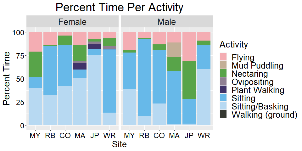
We conducted observations by releasing an individual and following it for up to 60 minutes. Each individual’s behavior was recorded and position marked with a pin flag every 15 seconds. Behavior types included flying, sitting, sitting/basking, nectaring, ovipositing, plant walking, mud puddling, and walking (on the ground), and mating. Some behaviors are sex-specific; only males exhibit mud puddling behavior, and only females oviposit and plant walk. Plant walking is a behavior exhibited when a female is attempting to select an oviposition site. She will crawl up and down the host plant before potentially choosing an oviposition site. We recorded which plant species individuals chose for nectaring, ovipositing, or plant walking.We randomly selected four points along each path to measure plant community data. Within a meter’s radius of each point, we measured host plant volume and counted flowering plant inflorescences. We used a Robel pole (Robel et al 1970) placed on the center point to obtain an index of vegetation height.
Data Analysis
All analyses were completed in the statistics program R. We used the package MoveHMM (Michelot et al 2016) to calculate the move lengths and turning angles from our GPS data. Following the methods in Kareiva and Shigesada (1983) and Turchin (1991), we calculated the expected net squared displacement and diffusion rate of each observed individual.
Question 1 Analysis
Using the silvery blue butterfly data, we ran a generalized linear mixed model (GLMM) with diffusion rates as the response variable, sex and management type as fixed effects and site as a random effect using the function glmer from the package lme4 (Bates et al 2015). The model used a Gamma distribution with a log link because the diffusion rates are bound by 0 and infinity but were skewed towards 0. Since the limited number of observations could make inference with a random effect more difficult, we also ran a generalized linear model (GLM) with the same response variable and explanatory variables but without a random effect of site using the glm function in the stats package (R Core Team 2021).
Question 2 analysis
Many blue (lycaenidae) female butterflies are known to be strongly associated with their host plants (e.g. Schultz 1998). Therefore, we tested for this using an a priori GLM with diffusion rates as the response variable and sex and mean host volume by species as explanatory variables, with a Gamma distribution and log link, using the glm function from the stats package (R Core Team 2021). For this analysis, we “binned” the Lupinus spp. host category because one of the species (Lupinus oreganus) was found at only one site (MA) and the other species (Lupinus albicaulis) was not found at the same site. Vicia sativa and Vicia hirsuta were kept as separate species.
We tested for effects of total host and nectar availability and vegetation height with a GLM. We used diffusion rates as the response variable and total host volume, total nectar inflorescence count, mean Robel index number, and sex as explanatory variables, again with a Gamma distribution and log link, using the glm function from the stats package (R Core Team 2021).
Preference/Performance Methods
COVID-Related Impacts: Due to restrictions on research and travel by WSU and Washington State in the wake of COVID-19, research plans were changed and we were limited to working in a single site. We focused on Riverbend Ranch because the site had the most significant changes to its management as part of its CGP treatment (introduction of rotational grazing and native seeding—see Appendix A, Figure 4). In addition, we were unable to access the pasture during parts of the season because of the cattle rotation on that site and the involved universities (WSU and The Evergreen State College) would not permit undergraduate interns or volunteers to participate in research in May 2020. Finally, an unusually wet and cool spring limited butterfly work because butterflies do not fly in cool, wet conditions. These factors together resulted in a substantially lower sample size than expected.
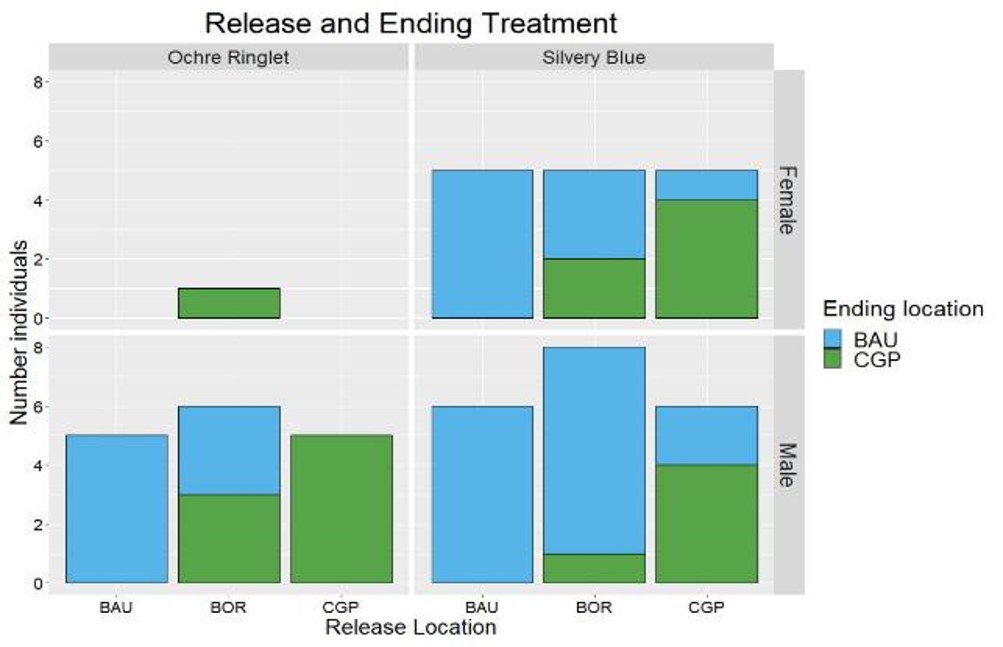
In 2020, we focused on comparing butterfly performance and butterfly behavior in CGP vs BAU. To measure edge behavior by silvery blue butterflies and ochre ringlets, we released butterflies at the boundary (BOR) of BAU and CGP and compared this behavior to releases at a “virtual” boundary of BAU and CGP (Ross et al 2005, Schultz 2012). We released individuals at haphazardly chosen locations in the CGP and BAU treatments as far from borders and fence lines as possible, as well as haphazardly chosen locations along the border between treatments (Figure 5).
To measure performance, we collected females of both species in the field and attempted to encourage them to lay eggs in captivity. Then we would have raised their larvae to third instar before placing them in the BAU and CGP treatments and tracking their growth, residence time, and ant tending interactions. However, the field house did not have adequate conditions for oviposition or larvae growth. Due to COVID travel restrictions we were unable to travel to and from WSU Vancouver to use the greenhouse and we were unsuccessful in raising enough larvae to conduct the “performance” part of the study.
Preference/Performance Analysis
We compared the number of individuals who stayed within the release location treatment (BAU or CGP) and the number of individuals who left the release location treatment to the number of individuals who entered each treatment from the border. We tested for significance within species and sex with chi-square tests using the chisq.test function from the stats package, followed by a chi-square posthoc test from the chisq.posthoc.test package (Ebbert 2019).
Forage biomass sampling
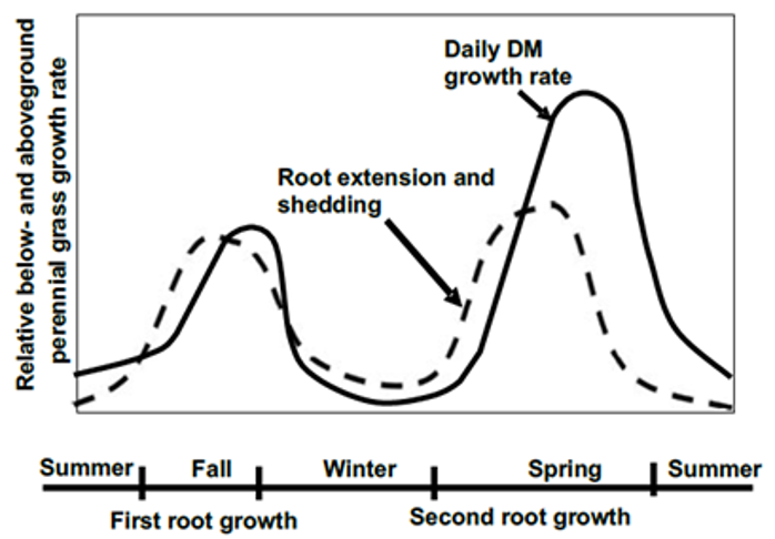
Timing and frequency of forage biomass and height estimations at prairie and ranch sites varied by site (Table 5). Sampling was designed around the seasonality of cool-season grass production (Figure 6) and deferment periods for native prairie plants to set seed. These two factors effectively identify key management periods (Figure 7), including an early season (February – March) grazing period prior to deferment, grazing deferment during native plant seed set (April – May/June), post-deferment grazing of stockpiled forage (June – July but as late as September), a roughly coinciding summer dormancy, a fall regrowth period (September – October), a late season grazing of fall regrowth where soil conditions permit, and finally winter dormancy when cool conditions limited further growth.
Table 5. Timing of biomass and height measures at grazed and ungrazed prairie sites in 2019.
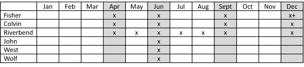
Rotational grazing management employed at Fisher and Colvin ranches. Rotational and continuous grazing employed at Riverbend where CGP included not only seeding but also a grazing paddock system. Total spring-summer biomass only was measured at ungrazed prairie sites (Johnson Point, West Rocky, and Wolf Haven)
Total forage biomass production at ranch sites was estimated by sampling at least four times in an attempt to capture a full picture of annual forage production. Each sampling period captured forage growth that occurred in the time since the previous sampling. Colvin and Fisher Ranches, which are rotationally grazed sites, were sampled in April, June, and December to capture early season, spring, and fall forage production, respectively. A post graze sampling (July – September) occurred to estimate ‘before-after’ forage presence to calculate utilization. The BAU (continuous grazing) and CGP (introduced rotational grazing paddocks) treatments at Riverbend were sampled monthly from April through September.
Prairie sites were sampled in June only, capturing forage growth during the primary growing season, after which point dry conditions effectively precluded further growth and forage dormancy began. Total biomass production at prairie sites was therefore based on June measurements.
At the ungrazed prairie sites, three of five 15 m x 15 m subplots within each replication were randomly
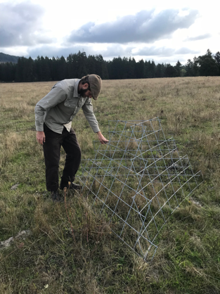
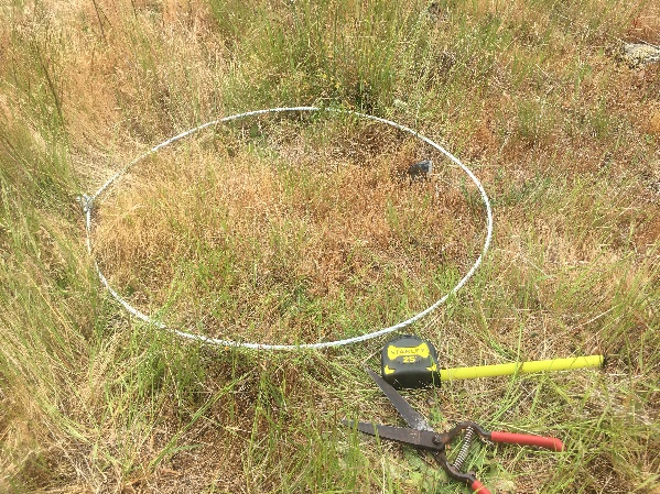
selected along a rough transect through each of six replications. One biomass sample was collected from each of the three subplots using a randomly tossed 0.45 m2 (4.8 ft2) cable ring (Figure 8). Aboveground plant material was clipped to ground level within each ring, creating a total of 3 sub-samples per replication. Sub-samples were dried at 55°C for five days at the WSU Puyallup Research and Extension Center. Dried weights were obtained to the nearest one-tenth gram and averaged to provide six replicate values per site (18 total measures, n=6).
Sampling at grazed sites utilized two grazing exclusion cages (Figure 9) per treatment (one in CGP, one in BAU). Each of the two cages was paired, at each time of sampling, with a no-cage sample randomly collected using the same cable method described above, providing a protected and unprotected biomass estimation (Figures 10, 11). Cages were used to detect any grazing that occurred prior to sampling (such as unplanned grazing in a site that should be in a rest period), as well as quantify cumulative biomass additions from the previous sampling (see below).

Total production and utilization measures relied on coordinated use of cage and no-cage samples. A cage-only or a cage/no-cage average in April provided the first production measure, onto which subsequent production estimates were added cumulatively. At the time of sampling, three cage forage heights, as well as a hoop biomass sample from within the cage were obtained. The hoop was then randomly tossed to a new location, and heights and a hoop biomass sample obtained. Then the exclusion cage was relocated directly adjacent to the no-cage hoop sampling site. Monthly cumulative biomass production additions were calculated by subtracting the no-cage hoop measure from the prior sampling periods from the cage hoop measure from the current sampling period, providing an estimation of the biomass added since the previous sampling.

April biomass at ranch sites contributed or did not to production based on whether cattle consumed detectable amounts. Summer (July/August) regrowth was analyzed specifically at Riverbend Ranch by shifting from measuring early season growth (dormant by late June) to the small amount of green post-graze summer regrowth (Figure 12), with the intent of tracking potential extension of forage production into the dry season in CGP treatments. Fall biomass production data were not yet analyzed at the time or reporting. Means comparisons were analyzed using JMP Pro Statistical Software (v15.2).
Forage height
At ungrazed prairie sites, three height samples were collected in each of three subplots used for biomass sampling. Starting from a reference point on the southwest corner (located by GPS) of each subplot, three height measures were collected at a series of 15-pace intervals in the directions north by northwest, then northeast, and then again north by north by northwest. Three height measures per subsample across three subplots across six replications were collected (36 total measures, n=6). Americorps members assisted with data collection for all vegetation, gopher, and forage metrics (Figure 13).
Forage height estimations at grazed sites were collected as noted in Figures 9 and 10, above. At cage locations, a measure was taken within each corner of the exclusion cage, while at no-cage locations, five measures were collected along a circle around the randomly tossed no-cage biomass sampling ring. Means comparisons were analyzed using JMP Pro Statistical Software (v15.2).
Biomass Utilization
Percent biomass utilization is reported here and is important to monitoring efficiency of forage use. However, it is complicated by potentially incomparable sampling methods, and high variability across sites, between treatments, and within experimental units. Some challenges were as follows:
- Monitoring continuous grazing using the cage method relied upon calculating the difference between cage and no-cage biomass (a spatial approach: a protected sample in one location, a second unprotected sample in another, taken during the same visit). Percent utilization can be estimated for each sampling period by dividing the biomass consumed (difference) by the total (caged). This measure averaged over every sampling period provided a season-long estimation of forage utilization.
- Monitoring rotationally grazed biomass relied upon calculating the difference between pre-grazed treatments (June sampling), and post-grazing (July September sampling), representing a temporal approach: post-grazing samples (remaining biomass) subtracted off pre-grazed samples (total available) to estimate forage consumed. In all cases reliable post-graze samples were difficult to obtain based on different grazing regimes and seasonal timing at the different ranches.
- While these are arguably the only available methods to compare percent forage utilization (spatial cage/no-cage and before/after) between these grazed systems, the methods are different, particularly in light of additional differences in overall biomass available in these systems at each time of sampling. Continuously grazed forage was between 0.6 cm and 7.6 cm (0.25 in and 3 in) tall, and biomass height in continuously grazed systems caged one month since the previous clipping was minimally greater. By comparison, rotationally grazed paddocks prior to grazing were 38 cm (15 in) and greater, while post-grazing paddocks in rotational systems remained 12.7 cm to 25.4 cm (5 to 10 in) in height with considerable variability from trampling and oxidation by post-graze sampling. In 2020 a post-graze sample at Colvin could not be obtained and thereby only April utilization could be estimated for that site-year.
Soil Quality Parameters
Soil nutrient assessment
Baseline soil nutrient status was evaluated in Fall 2018 from the three cooperating ranch sites and the three prairie sites. Where soil conditions allowed, fifteen ¾” soil cores from each replicate paddock/unit were obtained to a depth of 8 inches. In instances where rockiness prevented soil auger penetration, at least one exposed face soil sample from each quadrant of each replicate was collected to 8”. The exposed face consisted of exposing a vertical soil profile to 8”, which required an approximately 6” x 6” area excavation through gravelly conditions. Sub-samples from each replicate were combined, and a composite sample from each of the six replicates within each research site was sent to A&L Soil Testing Laboratories (Portland, OR) for analysis. Samples were refrigerated prior to shipping, then wrapped with gel packs in bubble wrap for transit. Samples were analyzed for nitrogen, phosphorous, potassium, calcium, magnesium, sulfur, iron, copper, zinc, manganese, boron, pH, cation exchange capacity, organic matter and estimated nitrogen release.
Soil samples were again collected at the completion of the research study in fall-winter 2021 using the same sampling protocol as described above. Samples were analyzed by A&L Soil Testing Laboratories. Differences between year, site, management (grazed/ungrazed), and treatment (BAU/CGP) were analyzed using JMP Pro Statistical Software (v15.2).
Soil Temperature, Bulk Density and Forage Dynamics
An evaluation of the relationships between forage height, soil temperature, grazing treatment and soil bulk density was added to the study in 2020. The research team was interested in the potential of higher residual forage in CGP treatments to decrease mean daily high soil temperatures, presumably due to shading effect, and thereby extend forage growth into the summer dormant period. This would be beneficial to ranchers.
Soil temperature data loggers (HOBO Pendant® MX 2201) were placed at 10cm depth in three replications in CGP and BAU treatments at Riverbend Ranch, and in three replicated plots at West Rocky Prairie. Temperature data was collected from late March through November 2020. Forage height was measured weekly, and soil temperature data was downloaded once per month.
Soil bulk density measures were obtained using an AMS Bulk Density Sampler Cup and AMS Compact Slide Hammer. Samples were collected in May and dried at 105°C for 72 hours. Bulk density was calculated as the dry mass per volume of the sampling ring (g/cm3). Means comparisons were analyzed using JMP Pro Statistical Software (v15.2).
Soil taxonomy work
Taxonomic soil descriptions were completed by the USDA Natural Resource Conservation Service Soil Survey staff operating out of Olympia, WA. One to three soil pits were excavated at each site; the number of pits depended on the presence or absence of mima mounds or low-lying topography. Both mound and intermound soil pits were dug on sites with mounds and pits were dug at other distinct landforms such as a low-lying area. Soil taxonomic work consisted of excavating soil with shovels to appropriate diagnostic horizons, which typically did not exceed 100 cm. Methods presented in the NRCS Field Book for Describing and Sampling Soils (version 3.0) were utilized to document site characteristics including parent material, landforms, land shape, and drainage, as well as diagnostic features (i.e., diagnostic horizons) and soil pit descriptions consisting of horizonation, color, texture, and structure (Table 2). Full soil taxonomic descriptions were included in a final report by NRCS staff.
Survey of Grazing Practices in Southwest Washington
We developed a survey using the Dillman survey design method (Dillman 2007) to gather information on grazing practices in western Washington, potential barriers and incentives to implementing conservation practices for landowners and feedback regarding regulatory programs and agency relationships. We asked two main questions: how do landowners perceive potential incentives and barriers to conservation? Which demographic and economic explanatory variables are most important in incentive and barrier perception?
The survey consisted of questions related to land use and land use history (multiple choice questions), conservation incentives and conservation barriers (Likert scale questions), conservation interest (Likert scale questions), relationships with agencies/organizations (Likert scale questions), and demographics (multiple choice questions). Respondents invited to share information they felt was not covered in the rest of the survey. Respondents were asked to indicate their level of interest in incentives to implement conservation strategies on a 5-point ordinal scale, from “1: No Interest” to “5: Extremely strong Interest.” Respondents were asked to indicate their perception of barriers to implementing conservation strategies on a 5-point ordinal scale, from “1: Not a barrier” to “5: Extremely strong barrier.”
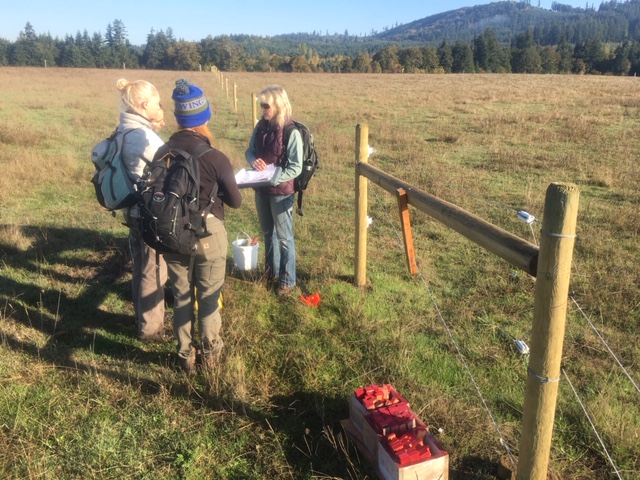
We vetted the survey through a meeting with a focus group comprised of three local producers and three project partners in Fall 2018. The producers each took the survey in draft form and then provided feedback on terminology, clarity, length, flow, and question relevance. We obtained the certificate of exemption from further review from Washington State University’s Internal Review Board in February 2019. We used a mixed method (Dillman 2007) to distribute the surveys online and in print. We built the emailed surveys through the survey software Qualtrics© and built the printed version in Microsoft Word.
Due to the relatively small number of potential respondents, we attempted a census of livestock owners within the counties of interest. We partnered with participating organizations throughout western Washington, including WSU county extensions, farm bureaus, conservation districts, and others, to distribute the survey via anonymous Qualtrics link to their email databases in April 2019. We were also able to obtain mailing addresses of some landowners through the Thurston and Lewis County Extension offices and mailed surveys to landowners for whom we did not have email addresses. Over 300 printed surveys were mailed in April 2019.
Survey Analysis
We tested the internal reliability of our scales using Cronbach’s alpha coefficient (Cronbach 1951; acceptable value > 0.6) using the psych package in R. We calculated an alpha coefficient of 0.85.
Question 1: Producer perception of incentives and barriers to implementing conservation
We compared producer perceptions of the incentives and barriers using an Extended Cochran-Armitage test due to the ordinal nature of the response variables. To increase our ability to detect differences among respondents, we recoded the response variable to a 3-point scale by collapsing the first and second levels and fourth and fifth levels, leaving level three as the neutral category. The response variable was analyzed as 1: Not interested, 3: Neutral, 5: Interested. Hereafter, when we discuss producer “preference” and “ratings” of incentives and barriers, we refer to the number of respondents interested in an incentive, or the number of respondents who rated an option as a barrier.
Question 2: Demographic and economic effects on producer perceptions of incentives
Following methods similar to Dalton and Jin (2018), we used ordinal logistic regression (OLR) to examine what effect demographic and economic explanatory variables had on producer perceptions of each individual conservation incentive and barrier. We used OLR because of the ordinal nature of the dependent variables. The relationship between the explanatory variables and the ordinal response variable is not linear, making linear regression inappropriate, while multinomial logistic regression does not account for the ordinal nature of the response variables (Liao 1994).
Our initial pool of explanatory variables included farm size, gross sales, and percent of income represented by the farm, age, gender, and education. Each incentive was analyzed separately; to make comparison possible between individual incentives, we needed to fit the same model to all. Due to a relatively limited number of responses and multicollinearity within the data, we excluded gross sales and percent income as they were correlated with farm size. We also combined levels in farm size and education.
To increase our ability to detect differences among respondents, we recoded the response variable to a 3-point scale by collapsing the first and second levels and fourth and fifth levels, leaving level three as the neutral category. Thus, the response variable was analyzed as 1: Not interested, 3: Neutral, 5: Interested. We fitted each model as:
![]()
Then we calculated the beta coefficient confidence intervals, the odds ratios (i.e. effect size), and p values. Due to rank deficiency within the data on perceptions of barriers to conservation, we were unable to analyze the barriers and Question 2 results are reported for farmer perception of incentives only.
Enterprise budgets
Enterprise Budget Development for Cattle Production
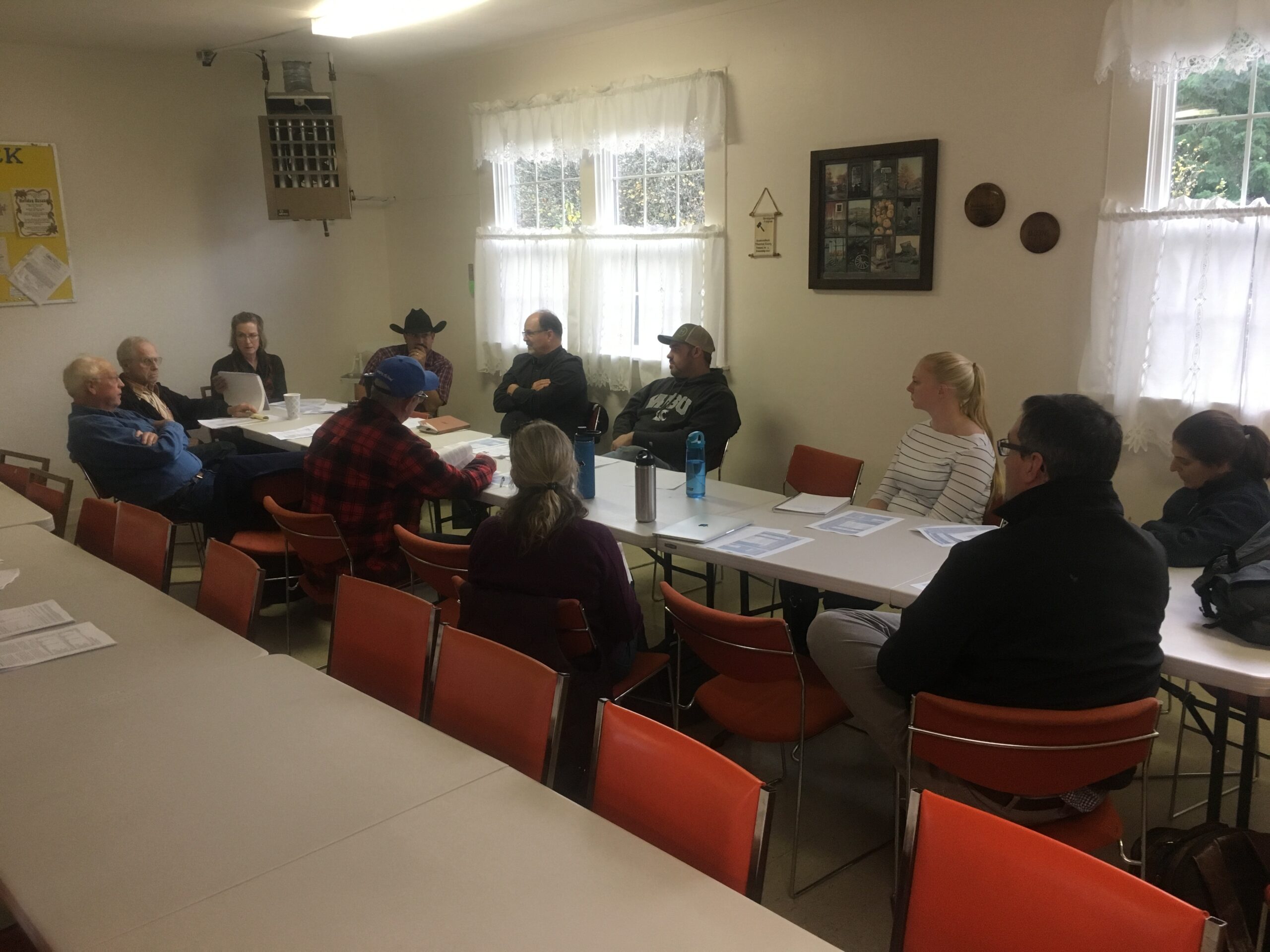
A meeting with producers was held for the purpose of conducting a Delphi Method survey of costs of cattle production in Thurston County. The DM is a formalized approach to assembling a group of experts and soliciting information in their area of expertise (Linstone and Turoff, 1975 and Weblar et al 1991), in this case, regarding the costs and earnings associated with various prairie grazing practices. Enterprise budgets were created that compare earning from traditional cow-calf production systems and grass-finished beef enterprises that market directly to consumers. In 2021, two enterprise budgets, a 50-head Cow-Calf and a Grass-Finished Steer, were finalized and reviewed by subject area specialists. These will be submitted as Extension bulletins in 2022.
Costs Estimates for Prairie Habitat Restoration Scenarios
A meeting with project personnel and stakeholders provided detailed scenarios for determining costs for three different prairie habitat restoration scenarios. These include Scotch Broom infested parcels, abandoned farmland, and abandoned rangeland. Specific annual operations for habitat restoration extend over multiple years. Relatively aggressive management is required to convert previously unmanaged land into prairie habitat with native species. Repeated burning, mowing, spraying and planting over many years would be required to restore these lands to their native status. These cost estimates were developed with input from Washington Department of Fish and Wildlife, Center for Natural Lands Management, Department of Natural Resources, and Ecostudies Institute. This work was led by Kathleen Painter at the University of Idaho. In 2021, three enterprise budgets were completed and used along with the grazing budgets to complete the Economic Impact Assessment.
Economic impact assessment
An economic impact analysis was undertaken to quantify the potential economic impacts of using different land management types to achieve species protection. The total economic impacts of five different combinations of ungrazed “new reserves” and grazed “working lands” acres were analyzed. An input-output analysis was developed using IMPLAN software to model the total new dollars introduced to the County and total economic impact of the five land management combinations.
To estimate economic impacts, enterprise budgets for grazing and restoration (above) were used to build a model of the expenditures (inputs) and sales (outputs) associated with the respective conservation programs. Given the enterprise budgets, the economic model was calculated by converting the expenditure functions from the enterprise budget data into percentages of the total expenditure that was made in each individual type of expenditure. These percentages represent the share of each dollar of output that goes to each type of expenditure. The expenditure categories from the enterprise budget data were bridged to the closest 3-digit NAICS sector using descriptions of the sectors provided by the U.S. Bureau of Economic Analysis (BEA).
Additionally, because some of the expenses included in the enterprise budget data were retail purchases, margins to select sectors were applied. Specifically, the “Other variable expenses”, “Fertilizer expense”, and “Fuel and oil expense” were assumed to be retail expenditures. To account for this a 25% retail and 25% transportation margin to the expenditure was applied (Steinback and Thunberg, 2006; Leonard and Watson, 2011).
Next the proportion of each dollar of output going into purchasing inputs from other local sectors of the economy was determined. The shares of the expenditure data from the enterprise budgets represent the gross absorption coefficients (GAC), which are defined as “value of the commodity purchased as inputs by regional industries expressed as a proportion of total dollar outlays for the particular industry” (Holland & Beleiciks, 2006.) However, before incorporation into a standard input-output model, gross absorption coefficients were purged of imports to represent regional absorption coefficients (RAC). To obtain the RACs, the GACs were multiplied by the regional purchase coefficient (RPC) for each respective input. RPCs are defined as the proportion of commodity demand from within a region that is met by supply from that same region. The RPCs used in this study were obtained from the Commodity Balance Sheet from IMPLAN; since RPCs are region-specific values, assumptions were made to identify representative counties from the national IMPLAN data for the appropriate geographies.
The first aspect of economic impact was estimated by calculating new dollars generated by each industry sector or program. For the sectors that were generated for this study, it was assumed based on the Thurston County HCP that all of the revenue for the NR sectors (abandoned range, and abandoned cropland, Scotch broom,) came from local sources (mitigation fees and property taxes for a land protection program known as Conservation Futures). This assumption implied that these sectors do not bring in new dollars to the region’s economy. However, it was assumed that the meat and livestock from the cow/calf and the grass-finished beef sectors (WLE) either sell their output outside of the county or sales within the county substitute for livestock/beef purchases that would otherwise consist of product imported from outside the county. Therefore, the sales of the livestock sectors were modeled as comprising new dollars in the regional economy (Cooke and Watson 2011).
Incorporating these assumptions, the impacts of all the sectors were estimated using an input/output model, described in more detail in a summary report: https://s3.wp.wsu.edu/uploads/sites/2056/2021/12/Economic-Impacts-Report_Final.pdf). Finally, economic multipliers were generated for each sector by relating industry output to changes in economic activity. The multipliers effectively quantify demand for industry outputs, and in plain terms economic value (or impact) generated by a new dollar bouncing through the local economy (within the defined study geography).
Seeded Species Establishment
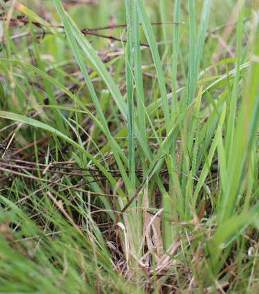
Out of the 10 species we seeded into CGP treatments, 5 successfully established in at least one CGP site by spring 2020 (as captured in our 1m2 quadrats): Castilleja levisecta (golden paintbrush), Collinsia parviflora (maiden blue-eyed Mary), Lupinus bicolor (bicolor lupine), Plectritis congesta (sea blush), Ranunculus occidentalis (western buttercup) (Figure 14). Presence of Collinsia parviflora and Lupinus bicolor in the BAU treatments was due to the fact they were already established at sites before seeding occurred (Table 6). The persistence of the annual species 2 years post-seeding shows that they are reproducing on their own in the CGP units. It is also worth noting that due to the patchy nature of establishment for some of the seeded species at the grazed sites, our monitoring quadrats did not capture their presence, despite large established patches in the paddocks. This is especially true for Cerastium arvense (field chickweed), which we found at both Fisher Ranch and Colvin Ranch (Figure 14).
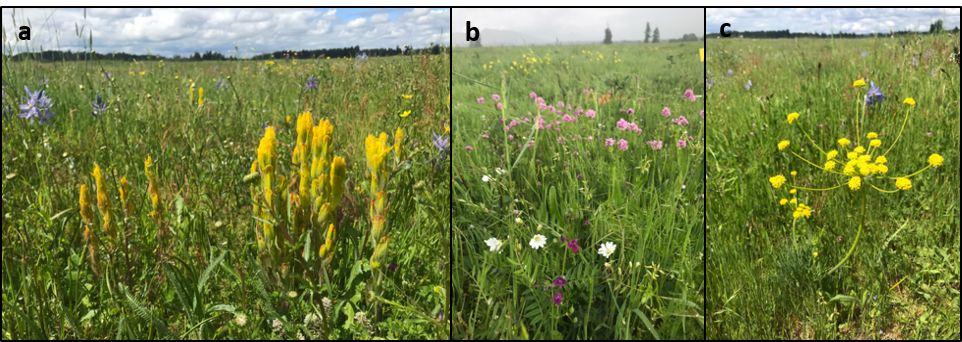
Table 6. Mean abundance of five of the native seeded species (± 1SD) across the different sites and the three treatments (n=6). Absolute abundance is quantified as the number of individuals per 1m2 monitoring quadrat. R. occidentalis was already present in large quantities at Colvin Ranch so it was not seeded, nor was it monitored there. This is represented by ‘N/A’.

Native Species Richness
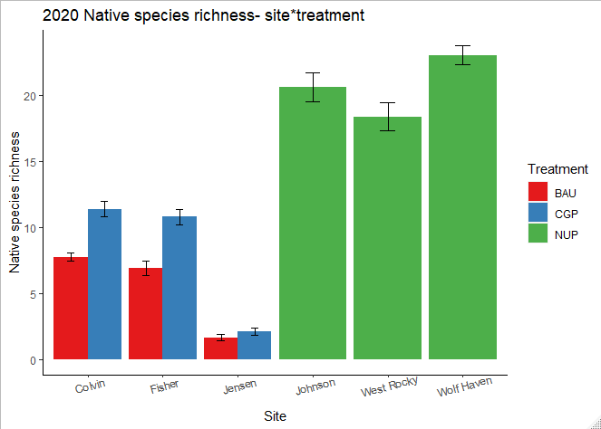
While the mean native species richness is still 4-5 times greater in the NUP than in either grazing treatment, the CGP treatments significantly increased native species richness over the BAU treatment within the first year of implementation (Figure 15, Table 7). Native species richness remained higher in the CGP treatments through 2020, despite no additional seeding in fall 2019. Sowing over multiple years and increasing seeding rates would likely further boost the establishment and persistence of native species.
Increased native species richness was observed within the CGP treatments at all ranch sites: Colvin gained five species, Fisher gained three species, while Riverbend gained one species (Figure 16). The increase in richness was due to the seeding of native species, in particular Plectritis congesta, Collinsia grandiflora, and Ranunculus occidentalis (Table 6). Compared to native ungrazed prairies, native species richness at ranch sites was much lower (2-12 species on average at ranch sites compared to 15-23 species on average in NUPs).
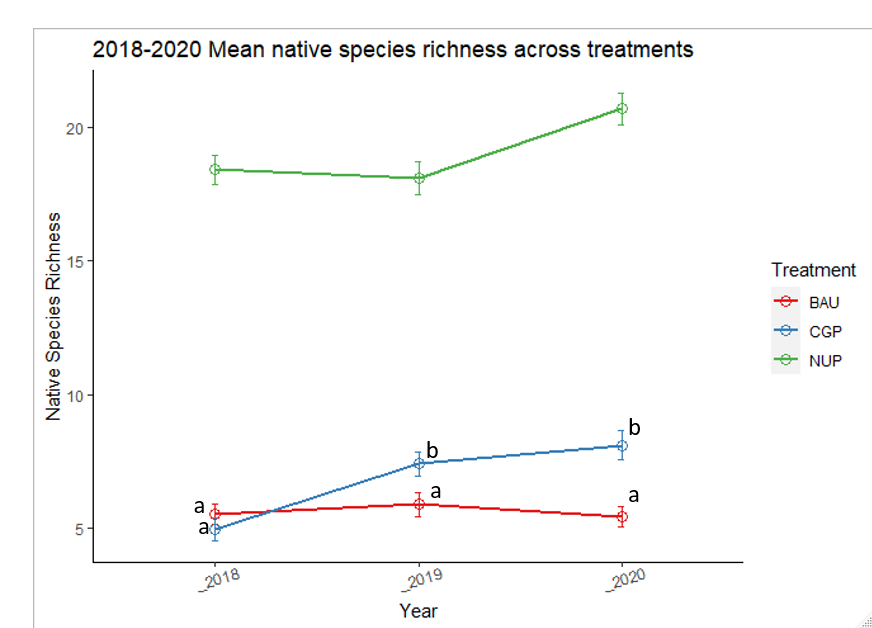
Table 7. Test statistics and p-values calculated from main effects and interactions within fitted models just between CGP and BAU treatments. Wald tests were used to calculate chi-square (c2) statistics and p-values for main effects. Interactions between year and treatment were calculated from Wald Z-tests for native forb cover and native species richness (GLMMs) and Wald t-test for non-native species richness (standard LMM). P-values in bold are considered significant at α=0.05.
|
Response Variable |
Year |
Site |
Treatment |
2019 Year*Trmt |
2020 Year*Trmt |
|||||
|
c2 |
p-value |
c2 |
p-value |
c2 |
p-value |
z/t value |
p-value |
z/t value |
p-value |
|
|
Native forb cover |
27.9 |
<0.001 |
64.2 |
<0.001 |
1.0 |
0.31 |
1.16 |
0.25 |
1.9 |
0.06 |
|
Native species richness |
65.4 |
<0.001 |
533.1 |
<0.001 |
15.1 |
<0.001 |
4.79 |
<0.001 |
7.8 |
<0.001 |
|
Non-native species richness |
116.2 |
<0.001 |
148.5 |
<0.001 |
3.7 |
0.05 |
0.08 |
0.93 |
5.4 |
<0.001 |
Percent cover of native forbs
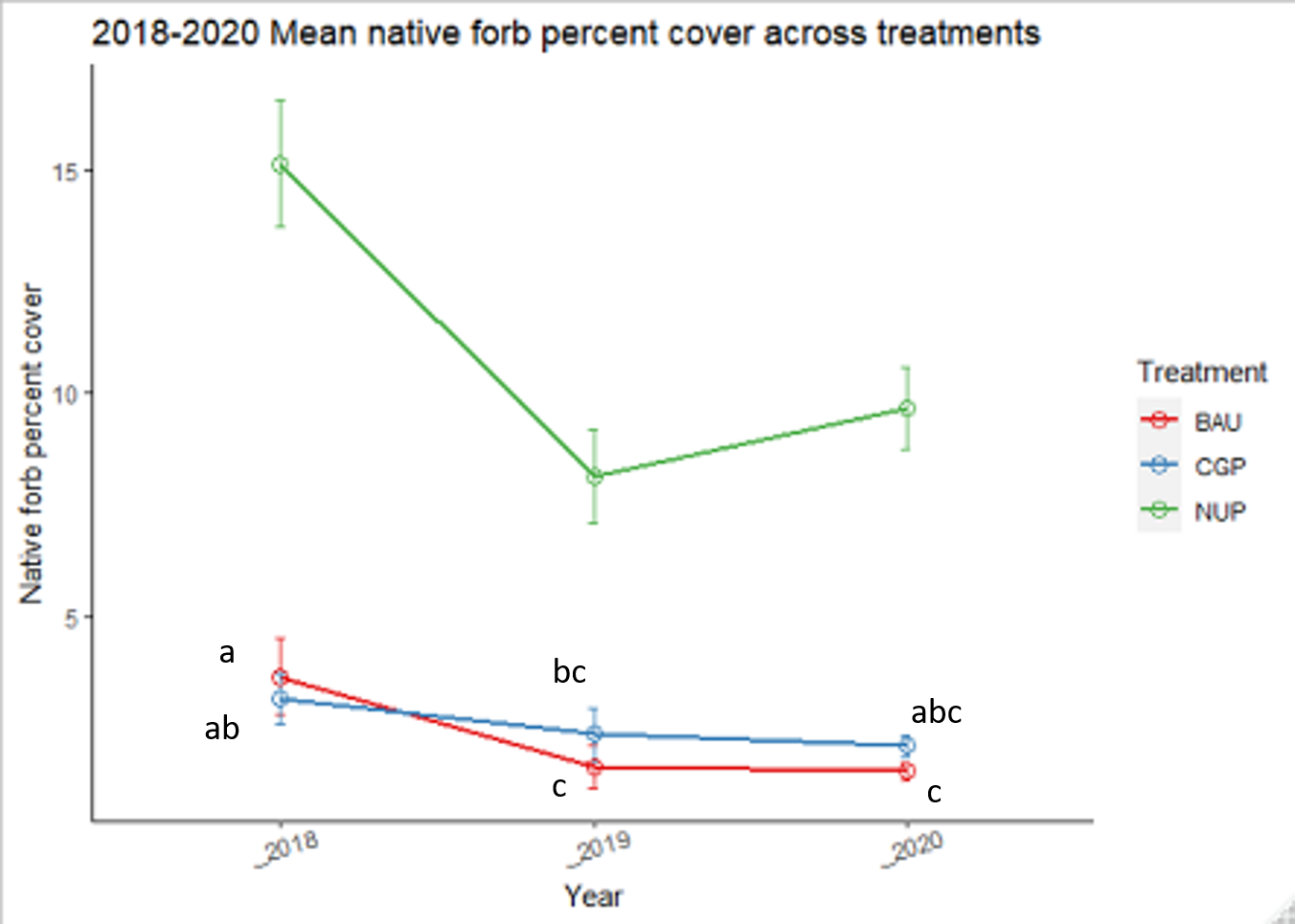
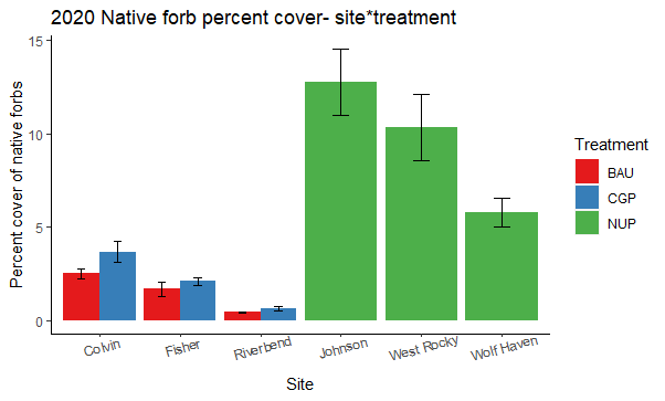
Two years after the implementation of conservation grazing practices (CGP), native forb cover showed minimal change within the CGP treatment and decreased slightly in the BAU treatment (dropping from 4% to 1%), though the effect of treatment was not significant (Figure 17, Table 7). Higher seeding rates of species that successfully established (Table 4) would likely have increased native forb cover in CGP treatments. Ranch sites varied in native forb cover, but all sites were <5% (Figure 18). In contrast, native forb cover was 2-3 times higher in native ungrazed prairies and fluctuated more over time.
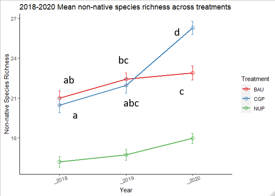
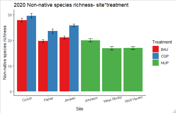
Non-native Species Richness
Non-native species richness showed minimal change from 2018 to 2019 but increased significantly in the CGP treatment in 2020 (Figure 19, Table 7). Both BAU and NUP treatments showed a slight increase in non-native species richness over time (~1.7 species on average for each treatment), but the CGP treatment gained an average of 6.2 species over the three years of the study. This surge was largely driven by increased richness at Fisher Ranch and Riverbend Farm (Figure 20), due to a mix of annual forbs and perennial grasses: Holcus lanatus, Medicago lupulina, Agrostis capillaris, Crepis capillaris, and Elymus repens.
Plant community composition over time
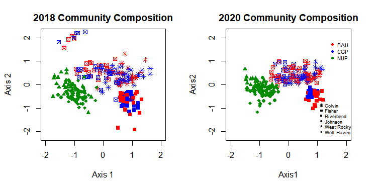
To visualize changes in plant community composition over time, we used non-metric multidimensional scaling (NMDS) ordination. This method clusters communities based on similarity so that assemblages that are more similar in species composition are closer together while those with disparate compositions are farther apart.
Overall, species composition across all plots became more similar from 2018 to 2020, as indicated by tightening of the plots across both Axis 1 and Axis 2 (Figure 21). Subsequent similarity percentage analysis (SIMPER) showed that Hypochaeris radicata, Plantago lanceolata, and Rumex acetosella increased in frequency across monitoring plots between 2018 and 2020, leading to increased similarity in composition. The native ungrazed prairie (NUP) sites all clustered together, reflecting similarity in composition. The ranch sites also clustered together more over time, with Fisher Ranch and Colvin Ranch hosting several plots with similar plant community compositions. Additionally, plant communities in the CGPs (blue shapes) have tightened along Axis 2, representing the native seeded species that have become established there.
Forage percent cover
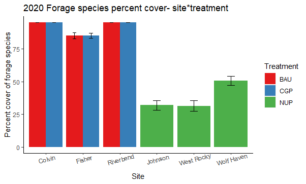
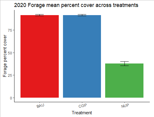
Forage cover was high at all ranch sites (>85%, Figure 23) with no detectable difference between the CGP & BAU treatments (p=0.9; Figure 24) two years after conservation grazing practices were implemented. Not surprisingly, forage cover was significantly lower on native ungrazed prairies (p<0.001; Figure 24).
Forage Cover Species Response to Conservation Grazing
Implementation of a rotational grazing system at one grazing site (Riverbend Ranch) afforded the opportunity to monitor forage cover responses to an introduced planned grazing regime. Cattle provided free and continuous access to fields are reputed to consume more tender, palatable species over time, resulting in stands dominated by short-lived, less palatable, and quick-reproducing species. These are presumed to consist of weedy annuals and perennials, and undesirable perennials such as Canada thistle (unpalatable), sub-terranean clover (smothers other desirable species), or other. By contrast, generating higher stocking rates on limited-area paddocks for short periods of time is understood to modify behavior by pressuring grazing livestock to forage less discriminately out of a degree of competition with the rest of the herd. In this forage cover sub-trial we evaluated the effect of CGP and BAU treatments on a variety of forage cover metrics including perennial cover and percent grass cover.
Inherent pasture heterogeneity across the grazing landscape reflected considerable micro-scale variability with the result that random effects from replication in many cases masked potential fixed effects of treatments. When all six replications for the experiment was analyzed, vegetation differences (percent grass cover and percent preferred grasses versus less preferred grasses) between the CGP and BAU treatments failed to rise to the level of significance (Table 8). Yet amidst significant vegetative variability between replications, emergent differences appeared to barely fail to rise to the level of significance, with the suggestion that vegetation dynamics appeared to be shifting to more preferred grass species after three years in an altered grazing regime in CGP.
To further explore this effect, several subsets of the full set of six replications were analyzed in an attempt to sift out treatment effects from swings in landscape patchiness (Table 9). This was done by running Student’s t-tests on uniform subsets of replications (i.e. 1-4 or 1-3), or by excluding the two replications with the highest percent cover preferred species from each treatment (which were not the same rep for each treatment). This amounted to excluding replication data where a handful of individual large plants dominated the count (i.e. high microsite variability). This patchiness on the landscape resulted in large swings in both CGP and BAU (note standard errors, Table 9). Excluding an even number of reps in each treatment where these large variations were observed (i.e. two BAU and two CGP treatments) allowed for a comparison of the remaining four reps with fewer outlying values.
We report this data because the emergence of trends in forage cover amidst considerable landscape heterogeneity appeared indicative of developing shifts in the forage community that were visibly apparent, particularly in persistent green cover in CGP treatments longer into dry summer months.
Table 8. Effect of Treatment on Forage Cover Metrics, All Reps
|
Cover or species metric (%) |
BAU |
CGP |
t Ratio |
Prob > t |
|
Annuals, cover |
38.5 |
36.4 |
-0.28 |
0.61 |
|
Annuals, species |
35.9 |
36.2 |
0.07 |
0.47 |
|
Perennials, cover |
58.6 |
59.3 |
0.09 |
0.47 |
|
Perennials, species |
58.8 |
58.9 |
0.01 |
0.50 |
|
All grasses, cover |
55.1 |
65.1 |
1.43 |
0.09 |
|
All grasses, species |
42.1 |
44.3 |
0.48 |
0.32 |
|
All forbs, cover |
44.9 |
34.9 |
-1.43 |
0.91 |
|
All forbs, species |
57.9 |
55.7 |
-0.48 |
0.68 |
|
More preferred grasses, cover |
11.0 |
18.5 |
1.07 |
0.15 |
|
Less preferred grasses, species |
32.4 |
45.1 |
0.87 |
0.20 |
Alpha values of less than 0.05 for Prob > t indicates probability that mean value of CGP is greater than BAU. Italicized bolded p-value denotes narrowly insignificant values.
Table 9. Effect of Treatment and Replication Variability on More Preferred Grass Cover (%)
|
Replications |
BAU |
|
CGP |
|
|
|
|
|
Mean (%) |
SE |
Mean (%) |
SE |
t Ratio |
Prob > t |
|
1-6 |
11.0 |
0.043 |
18.5 |
0.055 |
1.07 |
0.155 |
|
1-4 |
4.5 |
0.017 |
18.8 |
0.07 |
1.92 |
0.071 |
|
1-3 |
2.8 |
0.004 |
11.6 |
0.001 |
19.99 |
0.001 |
|
4 low |
4.5 |
0.017 |
10.2 |
0.013 |
2.68 |
0.020 |
Alpha values of less than 0.05 for Prob > t indicates probability that mean value of CGP is greater than BAU.
Gopher Occupancy
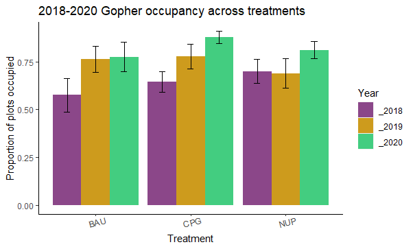
Gopher occupancy, measured as the proportion of plots with fresh gopher mounds present, increased over the project period at all sites except Johnson prairie. The greatest increase occurred in the CGP treatment (56% occupied in 2018 to 83% occupied in 2020; Figure 22). Interestingly, treatment was not a significant factor for predicting gopher occupancy in the fitted model (X2=1.8; p=0.41), suggesting that gophers can use habitat on grazed working lands at levels comparable to protected prairie preserves.
Forage biomass
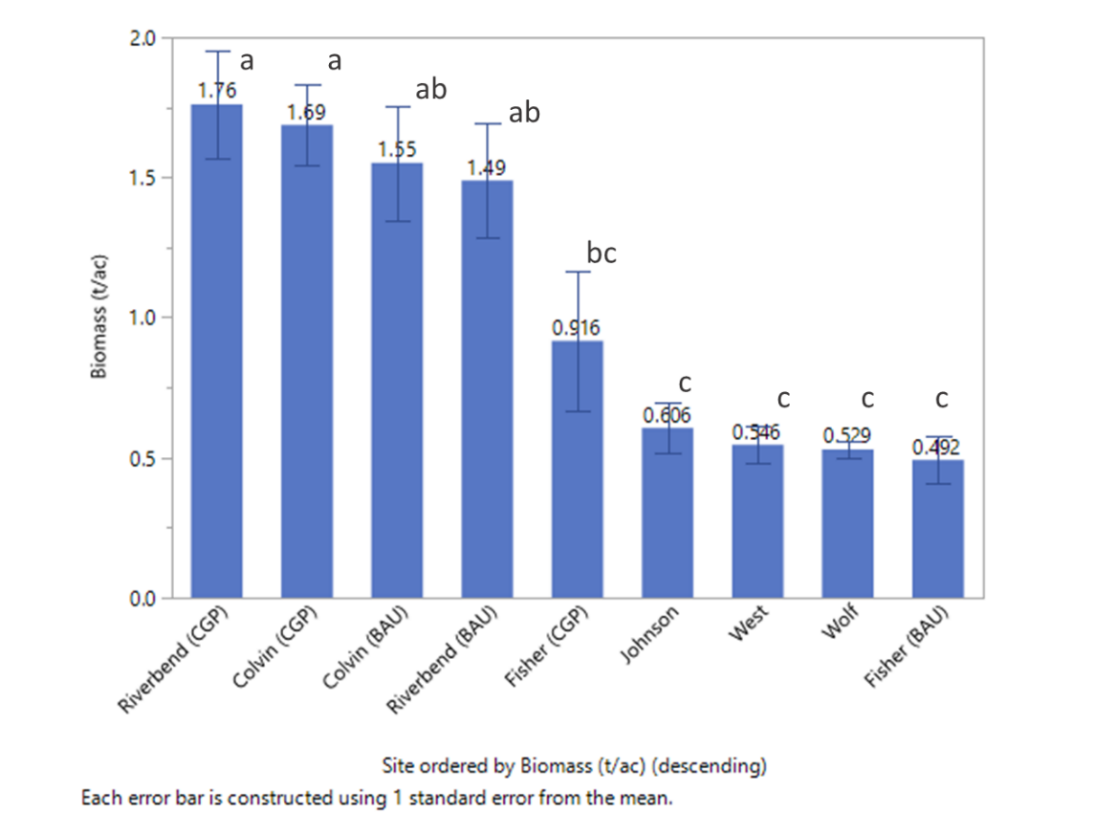
Biomass production ranged from 0.49 to 1.76 (2019) and 1.54 to 2.5 (2020) tons per acre for ranch sites, and from 0.53 to 0.61 (2019) and 0.48 to 0.58 (2020) tons per acre for upland prairie (Figures 25 and 26). The highlights of this work indicate that:
- Biomass production in all years was generally the highest and not significantly different across CGP and BAU treatments at the Colvin and Riverbend Ranch sites (Figures 25 and 26).
- CGP practices did not depress overall forage production and thereby native seeding is unlikely to negatively affect forage production in grazed systems.
- Significantly lower forage production was observed at Fisher Ranch, likely due to a combination of high stocking rate, shorter and inconsistent rest periods (data not shown), and lower soil fertility (Tables 15, 16, and 17).
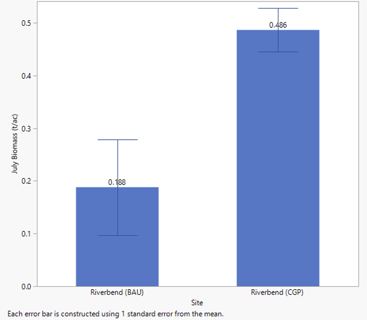
- Taller stubble height, and more regular rest periods resulted in greater forage production longer into the summer forage dormancy period in CGP as compared to BAU treatments (Figure 27).
- Early spring grazing prior to the deferment period effectively utilized spring forage availability in paddocks at Colvin Ranch, while lack of early spring grazing at Riverbend Ranch lowered overall utilization (wasted forage, Figure 28) by allowing grasses to become overly tall and mature during the grazing deferment.
Forage production at Riverbend and Colvin ranches were not significantly different. Due to higher stocking rates, Fisher Ranch was generally utilized fewer and shorter rest periods between grazing rotations, detected in significant cage/no-cage grazing differences during rest periods (data not shown). This resulted in lower biomass production (Figures 25 and 26). Additionally, low productivity at Fisher Farm is very likely also linked to lower phosphorus, potassium, calcium, magnesium, cation exchange capacity, and pH levels at this site (Tables 15, 16, and 17).
A notable dynamic in CGP treatments was the importance of utilizing spring forage prior to deferment. Missing this utilization as occurred at Riverbend depressed overall forage production below BAU at Riverbend, and lower than overall production as compared to Colvin Ranch generally. Nevertheless, CGP biomass totals were not statistically less than BAU totals, indicating no detrimental effect of seeding native species into pastures. In the future, improved spring biomass utilization in rotationally grazed fields at Riverbend combined with extended forage production into the summer may eventually yield greater forage productivity than continuously grazed fields.
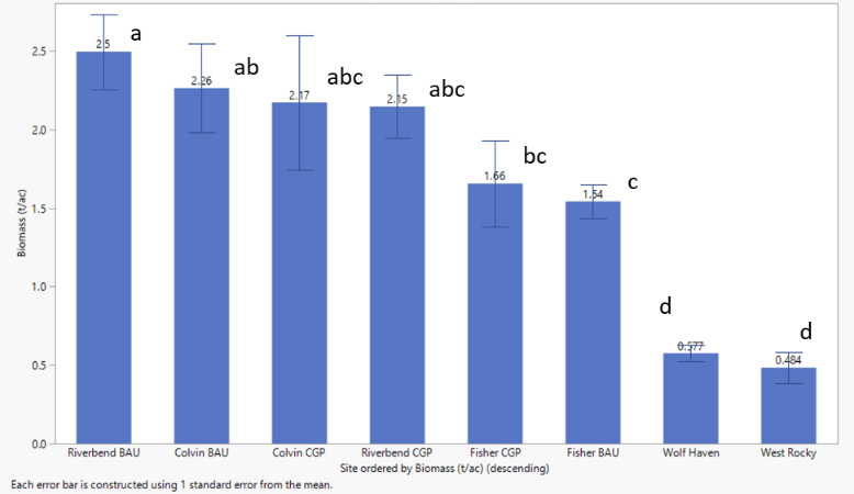
Lower biomass production at the ungrazed prairie sites (Johnson West Rocky, and Wolf Haven) in relation to Riverbend, Colvin and Fisher may be due to lower nutrient levels at these sites, in particular phosphorus, potassium, calcium, iron, and cation exchange capacity (Tables 15, 16, and 17). Another factor may be soil moisture. Forage and soils work in 2020 included forage quality assessment, soil compaction and soil temperatures, to evaluate the potential impacts of grazing generally, conservation grazing in particular, and lack of grazing on these forage quality and soil health parameters (see below).
In 2020 an expanded forage evaluation was developed to investigate the relationships between forage height, soil temperatures, and the potential to extend forage production further into the dry summer period when forage typically enters dormancy. Forage biomass aspects of this work are reported here and below under the section titled “Soil Quality Parameters”. Generally, CGP paddocks did exhibit the capacity to produce more, longer into the summer than BAU, as illustrated in significant differences in July biomass measured under exclusion cages in the two treatments (Figure 27).
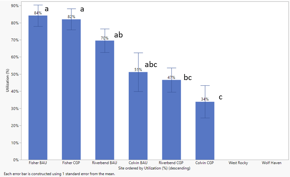
Forage Utilization
A take-half/leave-half approach to forage utilization is generally encouraged in rotational grazing systems. While it requires ranchers to forego usage, leaving forage allows for greater biomass productivity as a result. Percent forage utilization provides an indication of the extent to which this strategy is implemented by different ranch operations. As noted in the Methods section, utilization estimates were difficult to obtain due to considerable variability and differences in utilization data collection methods and calculations between rotationally and continuously grazed sites.
In 2020 forage utilization was apparently highest at Fisher and in BAU at Riverbend (Figure 28). Riverbend BAU and both Fisher treatments tended to exhibit very low stubble height (data not shown), high grazing pressure, and consequently high utilization rates. The 70-84% utilization rates in these systems effectively prevent robust root establishment and elevate daily average soil temperatures (Figures 35 and 36), which can delay regrowth in the spring and fall and lead to earlier forage dormancy in the summer dry season (Figure 27).
Relatively low utilization (47-50%) in Riverbend CGP reflected a better approach to conserving stubble, but also June/July forage trampling due to missed grazing prior to deferment. Given similar forage trampling was observed at Colvin Ranch, the higher utilization (62-73%) there in 2019 was unexpected. Utilization at Colvin in 2020 was only obtained for the spring rest period due to missing post-graze data. The lower March forage utilization rates (34-51%) reflect a modest and strategic use going into deferment.
Butterfly Movement and Behavior
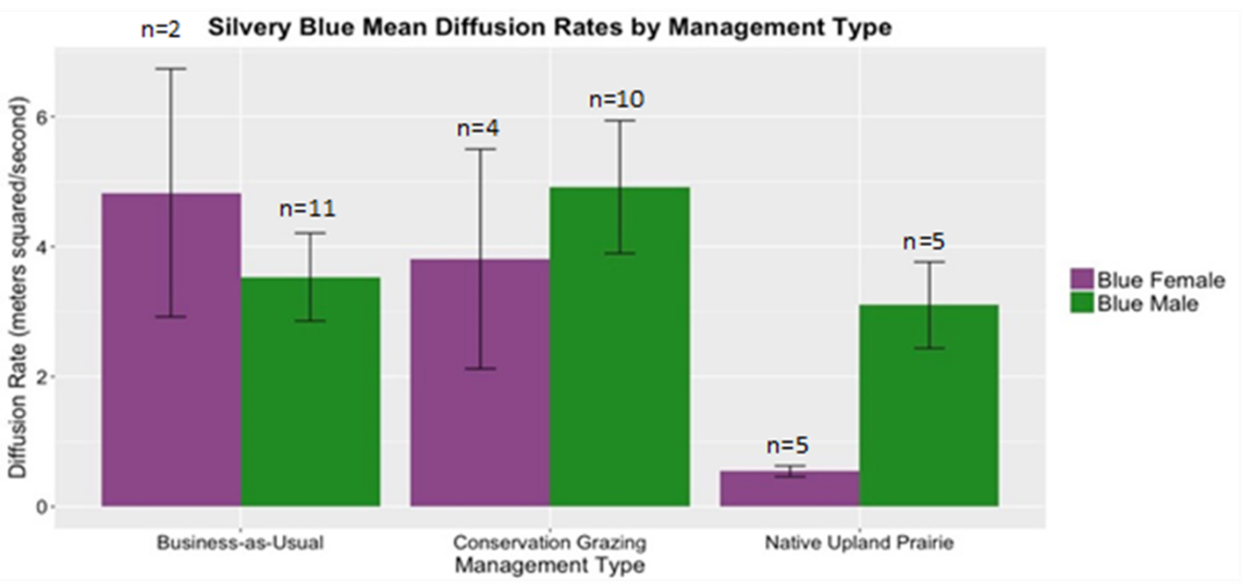
In Year 1, we observed flight paths for 11 female and 27 male silvery blue butterflies. We observed six female and 23 male ochre ringlet flight paths. Year 1 silvery blue female diffusion rates were lower in native habitat than conservation or conventional grazing but male movement behavior did not show a detectable difference (Figure 29a). Female silvery blue butterfly diffusion rates indicated concentrated search patterns exhibited in areas with high reward. Ochre ringlets did not exhibit a trend in diffusion rates across management types, regardless of sex (Figure 29b).
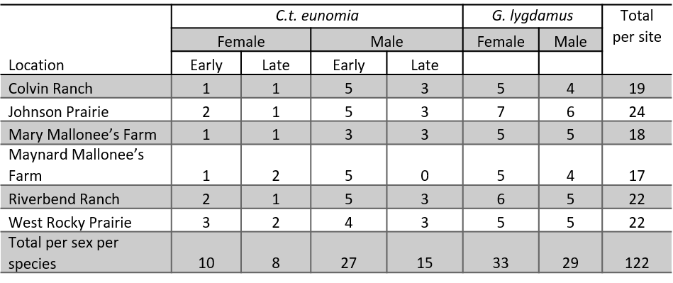
In Year 2, we observed 122 butterfly flight paths throughout the season (Table 10). Female ochre ringlets are more difficult to observe as they are skittish and sedentary. This limited the number of observations that could be completed. In the late season, weather limited progress, as it was unusually cloudy and extremely windy in the afternoons.
Table 10. The total number of observations in Year 2 per site separated by species and sex. Ochre ringlets are further separated by the flight period in which the observation was collected. The early flight ran May-July and the late flight ran July-September. Silvery blue butterflies have only one flight period (May), so the data are not separated by flight period.
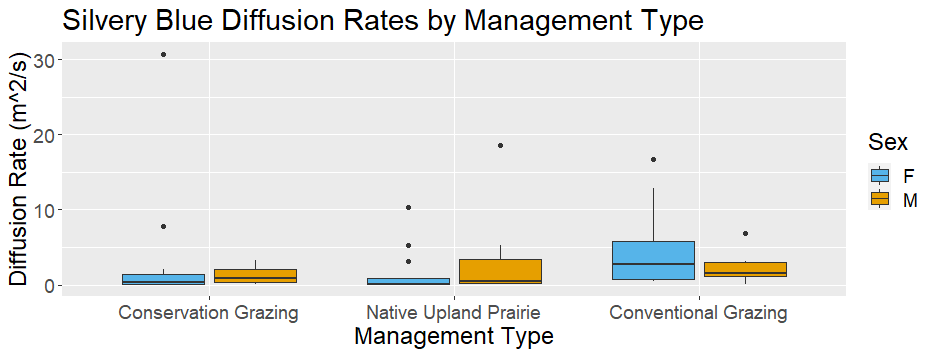
Question 1
We did not detect significant differences in silvery blue butterfly diffusion rates between management types with a GLMM (Table 11; Figure 30). We detected a nearly significant effect of the Native Upland Prairie management type on silvery blue butterfly diffusion rates with a GLM (Table 11; Figure 30). The estimated regression coefficient for Native Upland Prairie was negative, indicating that diffusion rates are lower in prairie habitat.
|
|
GLMM |
GLM |
|||
|
Predictors |
Estimates |
p |
Estimates |
p |
|
|
(Intercept) |
1.8056 |
<0.001 |
1.9814 |
<0.001 |
|
|
Conservation Grazing |
-0.5847 |
0.244 |
-0.5719 |
0.1513 |
|
|
Native Upland Prairie |
-0.6694 |
0.179 |
-0.6818 |
0.0813* |
|
|
Sex (Male) |
0.3537 |
0.163 |
0.2396 |
0.4534 |
|
|
Random Effects |
|||||
|
σ2 |
1.17 |
|
|||
|
τ00 |
0.19 site |
|
|||
|
ICC |
0.14 |
|
|||
|
N |
6 site |
|
|||
|
Observations |
62 |
62 |
|||
|
Marginal R2 / Conditional R2 |
0.082 / 0.208 |
0.137 |
|||
Question 2
We observed 40 total flowering plant species in bloom across the six sites throughout the silvery blue butterfly flight season (Appendix C). For ease of analysis, here we include only the 11 flowering plants that we observed silvery blue butterflies to nectar on (Figure 31a). We observed four host plant species across the six sites (Figure 31b).
The a priori GLM with host plants and sex as explanatory variables found a significant effect of Lupinus spp. volume and Vicia hirsuta volume on silvery blue butterfly diffusion rates (Table 12). The estimated regression coefficients for both Lupinus spp. and Vicia hirsuta were negative, indicating that greater volumes of those plants are associated with lower diffusion rates. There were no significant effects of nectar availability, vegetation height, or sex, but there was a significant effect of total host plant volume (Table 13).
Female silvery blue butterflies only oviposited on Lupinus spp. host plants but did oviposit in a grazed site (MA; Figure 32). We observed only one instance, which was not during a formal observation, of a butterfly walking on a Vicia sativa plant, indicating that the individual was considering oviposition, but she left the plant before doing so. Our next steps are to continue these analyses with the ochre ringlet diffusion rates and behavior.
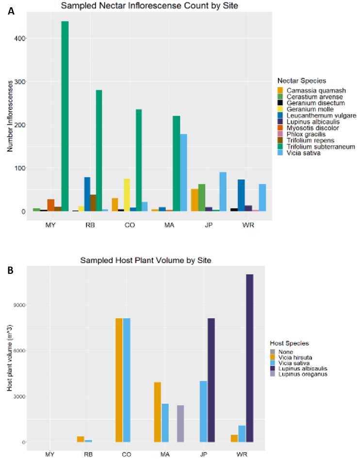
Table 12: An a priori model of mean host plant volume per path effects on silvery blue butterfly diffusion rates.
|
|
Diffusion Rate |
|
|
Predictors |
Estimate |
p |
|
(Intercept) |
5.83 |
<0.001 |
|
Lupinus spp. volume |
-1.345e-06 |
<0.001 |
|
V. sativa volume |
4.072e-07 |
0.384 |
|
V. hirsuta volume |
-9.098e-07 |
0.0435 |
|
Sex (Male) |
2.773e-01 |
0.327 |
|
Observations |
59 |
|
|
R2 |
0.479 |
|
Table 13: An a priori model with total host and nectar availability and vegetation height on silvery blue butterfly diffusion rates.
|
|
Diffusion Rate |
|
|
Predictors |
Estimate |
p |
|
(Intercept) |
2.055 |
<0.001 |
|
Total Host Volume |
-3.83e-07 |
<0.001 |
|
Total Nectar Count |
2.23e-04 |
0.848 |
|
Mean vegetation height (index) |
-0.166 |
0.204 |
|
Sex (Male) |
0.217 |
0.448 |
|
Observations |
59 |
|
|
R2 Nagelkerke |
0.370 |
|
Butterfly Preference
In 2020, we observed 52 total flight paths (Table 14). Chi-square tests indicated significant differences in the ending locations based on the starting location in silvery blue males and females and ochre ringlet males (p < 0.05; Figure 33). Post-hoc tests indicated that the significant differences were between the BAU and CGP release locations, which showed that individuals did not tend to move far enough to cross borders and were not attracted to CGP or BAU. There were no significant differences in path ending locations at the border release locations, indicating that individuals did not exhibit a preference for BAU or CGP.
Our next steps are to follow similar methods to the behavior/movement experiment to calculate the direction of movement, as well as flight path parameters (movement steps and turning angles) to quantify habitat-specific diffusion rates and compare them between BAU and CGP treatments, as well as to compare movement and movement directions at the border release locations.
Table 14: Number of successful behavior observations per release location by species and sex in 2020.
|
Release Location |
Ochre Ringlets |
Silvery blue butterflies |
||
|
Female |
Male |
Female |
Male |
|
|
Business-as-Usual |
0 |
5 |
5 |
6 |
|
Conservation Grazing Practice |
0 |
5 |
5 |
6 |
|
Border |
1 |
6 |
5 |
8 |
Butterfly results discussion
Greater host plant availability (especially large perennial Lupinus spp.) on a flight path level results in slower silvery blue butterfly diffusion rates, indicating that individuals perceive habitat with host plants as higher value habitat. Lupinus spp. host plants are often considered to be undesirable by farmers and ranchers as they are toxic to cattle and may cause pregnant cows to abort their fetuses (Panter et al. 2002). However, cattle generally will not eat Lupinus spp. unless they have no other choice (Stephen Bramwell, pers. comm), and we observed cattle to clip individual grass stems from under Lupinus plants without touching the plant itself (pers. observation). This observation fits with other studies that found cattle to promote greater plant community diversity and more nectar and host plant resources by reducing competitively dominant grass cover through foraging preferences (Wang et al. 2007; Zakkak et al. 2014; Delaney et al. 2016).
Silvery blue butterflies are common, relatively generalist species, so from their perspective, there may not be strong differences between the sites and management types apart from host plant availability. Even our “conventional” grazing pastures did not cover the full range of potentially negative grazing practices in the region, as producers willing to allow access to their land for butterfly experiments were already interested in conservation and were involved with the WSARE project. Two pastures in the behavior and movement experiment were certified organic farms (MA and MY), and the other two, regardless of grazing strategy, use little to no pesticides, which is not the case at all farms and ranches in the region. It is possible that we may have seen more of a contrast in behavior and movement rates if we had access to pastures that were more destructively grazed or used pesticides. In addition, silvery blue butterflies may be responding to an unmeasured or unanalyzed variable(s) in our system such as immediate weather conditions or microclimate variables.
Female silvery blue butterflies oviposited on lupines in grazed pastures, indicating that they recognize grazed pastures as habitat if their Lupinus spp. host plants are present. If butterflies will recognize grazed pastures as habitat if their host plants or other resources are present, then there is potential for grazed land to contribute to butterfly habitat in the landscape. Therefore, to support a wide range of butterfly species, grazing practices that support the greatest diversity of host plants should be encouraged, such as low intensity grazing with compensation to producers for lost income (Bussan 2022, Pöyry 2004, 2005, Weiss 1999). This conclusion does not apply to all butterfly species or grazed habitats. While we were fortunate to be allowed access to working farms and ranches, we were restricted to working with common generalist species, like silvery blue butterflies. Sensitive species may be more discerning in their behavior, movement, and habitat perceptions and may not respond to grazing in the same way as generalist species (Henry et al. 2019, Murphy et al. 2011).
Our butterfly preference experiment did not find evidence of preference for one treatment over another. Individuals of both species and of both sexes in silvery blue butterflies tended to stay within the treatment in which they were released. The slightly higher number of individuals who left CGP treatments may have been because of the smaller size of CGP paddocks; there was a higher chance of encountering a border. Additionally, there may not have been enough time since the beginning of the experiment to observe a strong enough signal from the plant community (Figure 15, 17) to be reflected in butterfly preferences and behavior in CGP and BAU treatments.
Soil Quality Parameters
Forage Heights, Soil Parameters and Soil Taxonomic Work
Soil nutrient status varied considerably between sites (Table 15), as well as by management type, at the outset of the study (Fall 2018). Soil nutrient levels tended to be generally higher under grazed as compared to ungrazed management, as observed in significantly (p < 0.05, Students t-test) higher levels of phosphorus, potassium, calcium, and magnesium in grazed systems (data analysis not shown). Sulfur levels were higher under ungrazed management, and pH, cation exchange capacity levels were higher under grazed management. No differences were observed in N03-N, or organic matter levels.
Table 15. Soils Nutrient Data Collection in 2018 as Expressed as the Sample Mean ± 1 Standard Deviation.

Table 16. Effect of Management and Experimental Treatments on Soil Fertility Parameters at Riverbend Ranch, Colvin Ranch, Fisher Ranch, Johnson Prairie, and Wolf Haven Prairie..
|
Soil test |
Management |
Treatment |
||||||||
|
(ppm, or noted) |
Grazed |
Un-grazed |
P > |t| |
P>t |
P<t |
BAU |
CGP |
P > |t| |
P>t |
P<t |
|
N |
2.78 |
3.17 |
0.58 |
0.29 |
0.71 |
2.6 |
3.0 |
0.63 |
0.31 |
0.69 |
|
P |
34.3 |
6.8 |
0.01 |
0.99 |
0.003 |
19.1 |
41.3 |
0.18 |
0.09 |
0.91 |
|
K |
88.2 |
51.8 |
0.01 |
0.99 |
0.01 |
90.8 |
85.6 |
0.84 |
0.58 |
0.42 |
|
Ca |
516.3 |
293.8 |
0.02 |
0.99 |
0.01 |
517.2 |
515.3 |
0.99 |
0.50 |
0.50 |
|
Mg |
64.9 |
44.2 |
0.07 |
0.96 |
0.04 |
67.6 |
62.2 |
0.76 |
0.62 |
0.38 |
|
S |
13.5 |
15.3 |
0.33 |
0.16 |
0.84 |
13.8 |
13.2 |
0.87 |
0.56 |
0.44 |
|
Fe |
17.2 |
12.7 |
0.03 |
0.98 |
0.02 |
17.0 |
17.4 |
0.90 |
0.45 |
0.55 |
|
Zn |
1.8 |
2.1 |
0.73 |
0.37 |
0.63 |
1.4 |
2.1 |
0.49 |
0.24 |
0.76 |
|
Cu |
0.2 |
0.3 |
0.34 |
0.17 |
0.83 |
0.2 |
0.2 |
0.67 |
0.34 |
0.66 |
|
Mn |
2.2 |
2.3 |
0.71 |
0.36 |
0.64 |
2.1 |
2.2 |
0.86 |
0.43 |
0.57 |
|
OM (%) |
15.5 |
16.2 |
0.75 |
0.37 |
0.63 |
15.4 |
15.7 |
0.93 |
0.46 |
0.54 |
|
CEC |
4.6 |
2.9 |
0.02 |
0.99 |
0.01 |
4.6 |
4.6 |
0.95 |
0.52 |
0.48 |
|
pH |
5.4 |
5.3 |
0.75 |
0.62 |
0.38 |
5.4 |
5.4 |
0.91 |
0.45 |
0.55 |
*Bold font indicates significantly different pairs (p < 0.05, t-test).
Differences soil nutrient parameters also varied significantly by site (Table 17). Nutrient levels were generally highest at Riverbend and Colvin Ranch, with soil nutrient parameters for Fisher Ranch often clustered with the ungrazed prairie sites (Johnson Prairie and Wolf Haven prairie).
Table 17. Effect of Site on Soil Fertility Parameters at Riverbend Ranch, Colvin Ranch, Fisher Ranch, Johnson Prairie, and Wolf Haven Prairie.
|
|
Grazed |
Ungrazed |
|||
|
|
RB |
CR |
FR |
JP |
WH |
|
N |
1.0 (c) |
4.8 (a) |
2.5 (b) |
2.7 (b) |
3.7 (ab) |
|
P |
59.3 (a) |
42.7 (ab) |
1.0 (c) |
11.7 (bc) |
2.0 (c) |
|
K |
153.5 (a) |
69.2 (b) |
41.8 (c) |
58.3 (bc) |
45.3 (bc) |
|
Ca |
849.5 (a) |
550.5 (b) |
148.8 (d) |
324.7 (c) |
263.0 (cd) |
|
Mg |
98.8 (a) |
75.3 (b) |
20.5 (d) |
43.3 (c) |
45.0 (c) |
|
S |
5.8 (d) |
13.2 (c) |
21.5 (a) |
14.0 (bc) |
16.7 (b) |
|
Fe |
15.5 (b) |
24.2 (a) |
12.0 (b) |
13.7 (b) |
11.7 (b) |
|
Zn |
0.4 (c) |
4.0 (a) |
1.0 (c) |
3.0 (ab) |
1.2 (bc) |
|
Cu |
0.2 (ab) |
0.3 (a) |
0.1 (b) |
0.4 (a) |
0.3 (ab) |
|
Mn |
1.2 (c) |
3.3 (a) |
2.0 (bc) |
2.7 (ab) |
2.0 (bc) |
|
OM (%) |
6.1 (c) |
24.0 (a) |
16.5 (b) |
14.7 (b) |
17.7 (b) |
|
CEC |
6.7 (a) |
5.2 (b) |
1.9 (c) |
3.0 (c) |
2.7 (c) |
|
pH |
5.9 (a) |
5.3 (b) |
5.0 (c) |
5.4 (b) |
5.3 (b) |
RB = Riverbend, CR = Colvin Ranch, FR = Fisher Ranch, JP = Johnson Prairie, WH = Wolf Haven Prairie
Non-overlapping letters denote significant differences between site (p < 0.05, Fisher’s LSD).
Soil Temperature, Bulk Density and Forage Dynamics
Grazing treatments (CGP and BAU) and site management (grazing as compared to no grazing) were evaluated for their effect on residual biomass (i.e. stubble height) and soil parameters including soil bulk density and soil temperature. Stubble height and soil temperatures are illustrated in Figures 33 and 34. The goal of this evaluation was to understand potential impacts of stubble height on soil temperature, both from the point of view of climate resilient grazing systems, and for the potential of conservation grazing management to extend forage production into the warm dormant season by means of cooler soil temperature. Significantly different stubble heights were observed between sites (West Rocky, Riverbend) and grazing treatments (CGP = 5.72 in, BAU = 2.00 in; p < 0.05, Student’s t-test).
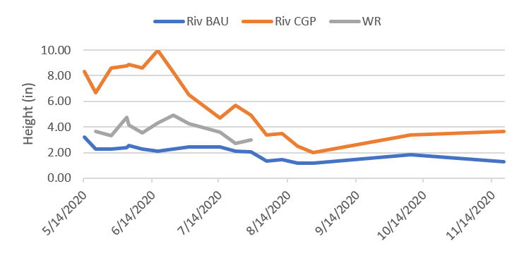
Significant differences in soil temperatures were also observed (Figures 35 and 36) between sites and treatments. Soil temperatures were highest at West Rocky Prairie and lowest in Riverbend CGP plots (highest stubble height), with soil temperatures in Riverbend BAU plots in the middle. Mean soil temperatures were 69.5 F (West Rocky), 67.4 F (Riverbend BAU), and 65.1 F (Riverbend CGP). Grazing events in which forage height was reduced appear to have led to temperature increases in CGP plots in relation to West Rocky.
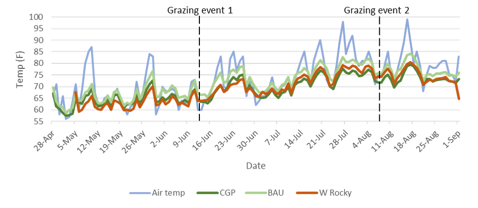
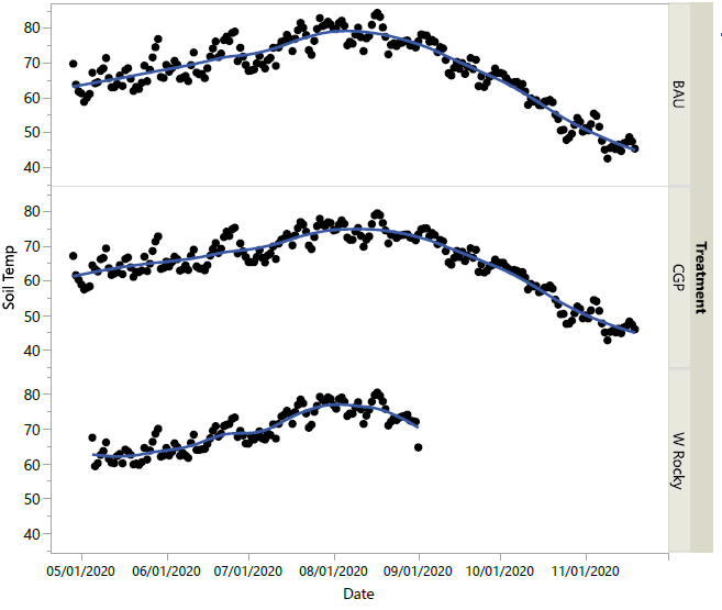
Higher stubble height management, and consequent shading effects, may have a beneficial impact on forage growth by decreasing summer average daily high soil temperatures. Significantly greater July biomass observed in CGP as compared to BAU cage samples (see Figure 26) illustrate the mitigating effect of higher forage heights on soil temperatures under CGP management.
Soil Bulk Density
Soil bulk density vales were obtained from CGP and BAU treatments at Riverbend Ranch. Mean bulk density in CGP and BAU were 1.14 g/cm3 and 1.15 g/cm3, respectively, and were not significantly different (data not shown). Typical bulk density values for moderately grazed sites are reported to be 0.9 g/cm3 (Engels n.d), indicating Riverbend sites (BAU as well as CGP) with a history of continuous grazing exhibit soil compaction. While we were not able to demonstrate that pasture rest associated with the CGP treatment decreased bulk density, it is possible that the duration of the study was insufficient for shifts in soil bulk density to occur.
Soil taxonomic work
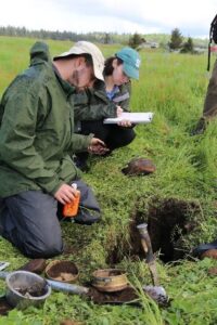
Regarding soil taxonomy, the majority of soil profiles at ranch and prairie preserve sites classified as either a Spanaway (Typic Humixercept) or Nisqually (Pachic Humixerept) series, or a higher-taxa of Pachic Humixercept (i.e., there is no existing soil series that would be a good fit). In general, the Spanaway-like soils were found in intermound areas, and the Nisqually-like soils were found on the mound sites that had a deeper, darker surface horizon(s). The higher-taxa Pachic Humixerepts, were described as Loamy-skeletal as compared to the sandy Nisqually, or sandy-skeletal Spanaway, meaning it had slightly more clay content within the control section. One outlier was a poorly drained, Norma soil found near a drainage ditch on one of the ranch research sites.
Based on these sites, a fairly clear pattern of deeper, more organic rich surface A horizons found on mounded areas and thinner A horizons found in the intermound position emerged. In addition, the mounded areas generally had either less rock fragment content by volume and/or smaller rock fragment diameter within the surface A horizons. In general, soil pit descriptions mostly conformed (though did not capture the higher taxa) to soil units mapped on NRCS Web Soil Survey (Table 18). Full soil pit descriptions are available upon request.
Table 18. Mapped soil series and soil series as verified by soil pit descriptions at ranch and prairie preserve research sites.

Survey of Grazing Practices in Southwest Washington
We received a total of 133 responses, 95 of which were from the emailed link and 38 from the printed surveys. Eighty-nine of the responses were from producers who have livestock and 39 were from producers who do not. Five respondents did not answer the question about whether they had livestock. As respondents could choose not to answer individual questions, response numbers per question varied. Twenty-two respondents owned or leased grazing land in Thurston County, 28 in Pierce County, 23 in Lewis County, and 13 in other counties. Full questionnaire results are available in the supplementary Survey Report.
Question 1: Producer perception of incentives and barriers to implementing conservation
Tax incentives and on-farm cost-share programs were the most preferred incentives (chi-squared = 64.024, p << 0.05), followed by conservation easements and transfer/purchase of development rights (Figure 1). Selling property for restoration/conservation or registry/branding certification programs were the least preferred (Figure 37).
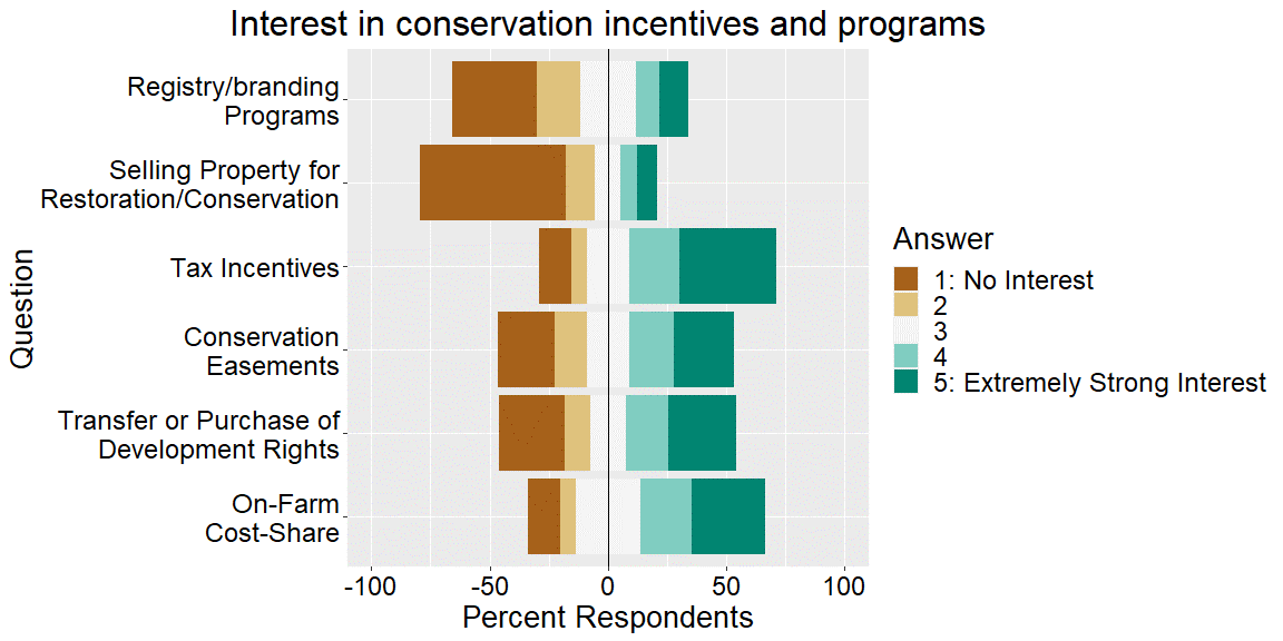
“Loss of development rights if listed species found” and “Not enough financial assistance available” were the most highly rated barriers (Figure 36), followed closely by “Not enough technical assistance available” and “Conservation is too expensive” (chi-squared = 63.369, p-value << 0.05) Social stigma was the lowest rated barrier to implementing conservation grazing (Figure 38).
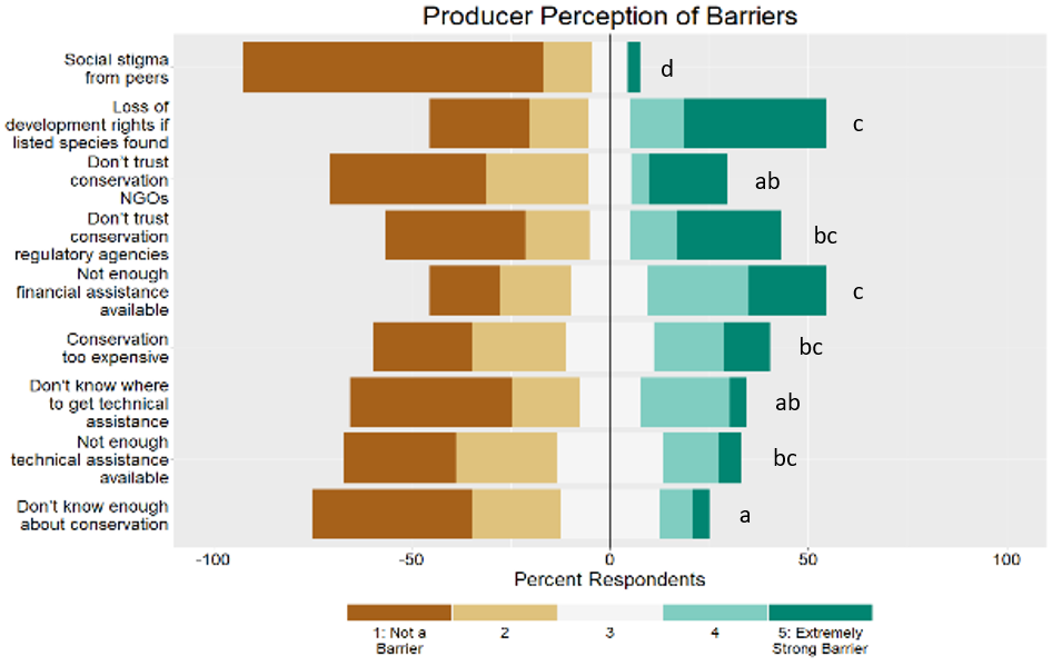
Question 2: Demographic and economic effects on producer perceptions of incentives
Respondent age and education level consistently played a strong role in determining incentive perception (Figure 39). Respondents in the oldest age category (70+ years old) tended to be less interested in all of the incentives than respondents in the 30-49 and 50-69 age categories. Respondents with associate, bachelor’s, or advanced degrees tended to be more interested in the incentives than those without education beyond high school. Farm size was important in perceptions of on-farm cost-share programs. Respondents in the largest farm category (300+ acres) were not interested in cost-share programs, while respondents in the next largest (100-299 acres) were interested (Figure 39).
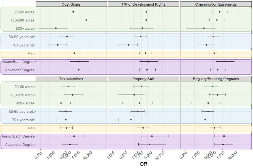
Cow-Calf, Grass Finished Beef, and Restoration Enterprise Budgets
Completed enterprise budgets for both grazing operations and ungrazed restoration operations are available on the project website: https://extension.wsu.edu/thurston/agriculture/on-farm-conservation/prairie/. Annual operational costs on a 50-acre basis for habitat establishment on abandoned cropland, abandoned rangeland, and Scotch broom infested land were $15,399, $15,818, and $21,339, respectively. No income was derived from these operations so no profit-loss figures were generated.
Annual net returns over total costs for a 50-head cow-calf operation in South Puget Sound were ($29,737) for the herd and ($595) per head. Discounting labor and fixed cost recovery, as is not uncommon in the region resulted in annual net returns over total costs of $3,880 for the herd, and $78 per head. Operations assumed 2 acres per head. Growing steers out over the approximately 30-month period to produce grass finished beef resulted in annual net returns over total costs for a 50-head operation of $5,151 for the herd, and $215 per head when marketing as quarter, half, or whole through WSDA custom exempt slaughter and processing. Marketing as USDA-certified generated annual net returns over total costs of $32,497 for the herd, and $1,354 per head.
Economic Impact Analysis
This study quantified the economic impacts of five scenarios (Table 19) that represent varying utilization of working lands (as either cow-calf or grass-finished beef operations) for species protection in the Thurston County Habitat Conservation Plan (HCP).
Table 19. Model Scenarios Identifying Acreage Mixes of New Reserves and Working Lands Easements to Protect, Enhance and Manage Habitat for the Covered Species
|
Model Scenarios |
New Reserves1 (ac) |
Working Lands Easements 2,3 (ac) |
Total (ac) |
|||||
|
Total acreage: 3,469 |
Total Reserve |
Abn-Crp |
Abn-Rgn |
Sct-Brm |
Total Working |
Cow-calf |
Grass-finish |
|
|
100% |
33% |
33% |
33% |
100% |
80% |
20% |
||
|
Draft HCP |
2,689 |
896 |
896 |
896 |
400 |
320 |
80 |
3,089 |
|
Scenario 1 |
3,469 |
1,156 |
1,156 |
1,156 |
0 |
0 |
0 |
3,469 |
|
Scenario 2 |
3,069 |
1,023 |
1,023 |
1,023 |
400 |
320 |
80 |
3,469 |
|
Scenario 3 |
2,469 |
823 |
823 |
823 |
1,000 |
800 |
200 |
3,469 |
|
Scenario 4 |
1,969 |
656 |
656 |
656 |
1,500 |
1,200 |
300 |
3,469 |
1New reserves starting point split evenly as “abandoned cropland (Abn-Crp), Abandoned rangeland (Abn-Rgn), and and Scotch broom (Sct-Brm)
2Working lands split 80:20 cow-calf and grass finished steer
3Easements set up using grazing budget
Sales from the livestock sectors introduced ‘new’ dollars into the region through the sale of product outside of the region or substitution of locally produced product (like beef) for imported product. New Reserve (NR) sectors in the baseline model run did not introduce new dollars into the region because all funding for these sectors (new prairie preserves established on abandoned range, and abandoned cropland, or Scotch broom) were projected by Thurston County to be funded locally from mitigation fees (on developers) and other sources (i.e. Conservation Futures taxes). As a result, total economic impacts increased when more working lands were recruited into the program ($0 with no working lands in Scenario 1 to $2.09 million with 400 ac working lands in Scenario 2, and $7.83 million with 1,500 ac of working lands in Scenario 4; Table 20).
Table 20. Economic Impacts‡ of the Respective Scenarios with Baseline Assumptions
|
Scenario |
Abandon Cropland |
Abandon Range |
Scotch Broom |
Conservation Partial |
Cow calf operation |
Grass finished livestock |
Total Impact |
|
Draft HCP |
0 |
0 |
0 |
0 |
$1,095 |
$993 |
$2,088 |
|
Scenario 1 |
0 |
0 |
0 |
0 |
0 |
0 |
0 |
|
Scenario 2 |
0 |
0 |
0 |
0 |
$1,095 |
$993 |
$2,088 |
|
Scenario 3 |
0 |
0 |
0 |
0 |
$2,738 |
$2,483 |
$5,221 |
|
Scenario 4 |
0 |
0 |
0 |
0 |
$4,107 |
$3,724 |
$7,831 |
‡Figures reported in 1,000s
Assuming 25% of NR funding could somehow be sourced externally increased total economic impacts ($688 thousand in Scenario 1, $3.60 million in Scenario 2, and $11.65 million in Scenario 4; Table 21). Generally, we found that total economic impacts uniformly increased, and costs decreased, in scenarios where greater proportions of working lands easements (WLE) were engaged.
Table 21. Economic impacts‡ the respective scenarios with the 25% exogenous restoration funding assumptions
|
Scenario |
Abandon Crop |
Abandon Range |
Scotch Broom |
Conservation Partial |
Cow calf operation |
Grass finished livestock |
Total Impact |
|
Draft HCP |
$157 |
$163 |
$198 |
$917 |
$1,095 |
$993 |
$3,523 |
|
Scenario 1 |
$202 |
$210 |
$256 |
$0 |
$0 |
$0 |
$668 |
|
Scenario 2 |
$179 |
$186 |
$226 |
$917 |
$1,095 |
$993 |
$3,597 |
|
Scenario 3 |
$144 |
$150 |
$182 |
$2,293 |
$2,738 |
$2,483 |
$7,989 |
|
Scenario 4 |
$115 |
$119 |
$145 |
$3,439 |
$4,107 |
$3,724 |
$11,649 |
‡Figures reported in 1,000s
Regarding restoration costs, these uniformly decreased in scenarios where greater proportions of WLE were engaged ($1.43 million in Scenario 1 with no working lands; $812 thousand in Scenario 4 with 1,500 acres WLE; Table 22).
Table 22. Other Economic Implications of Different Model Scenarios
|
Restoration Costs ($) |
Livestock Production Costs ($) |
Tax Revenue from Livestock Production ($) |
|
|
Draft HCP |
1,109,000 |
1,199,000 |
104,000 |
|
Scenario 1 |
1,430,000 |
0 |
0 |
|
Scenario 2 |
1,266,000 |
1,199,000 |
104,000 |
|
Scenario 3 |
1,018,000 |
2,997,000 |
260,000 |
|
Scenario 4 |
812,000 |
4,496,000 |
390,000 |
While WLE acquisition and restoration costs were lower than for NR acres, habitat value between WLE and NR are not equivalent (Bramwell et al. 2021). Higher NR acquisition and restoration costs may be justified in the Thurston County HCP by higher habitat values designed for and needed from NR acres. This economic data is intended only to help optimize the balance of WLE and NR acreage used in the HCP by weighing economic costs and benefits of utilizing each land type with respective habitat value costs and benefits.
Private tax revenue generated by working lands retained on the tax base while participating in the County HCP increased when more working lands acreage was recruited ($0 in Scenario 1 and $390 thousand in Scenario 4). Economic multipliers for cow-calf (2.05) and grass-finished beef sectors (2.51) were higher than economic multipliers for New Reserves established on Scotch broom (1.80), abandoned range (1.92), or abandoned cropland (1.90) due to higher rates of local re-spending in the livestock sectors. Scenarios overall exerted minimal impact on job creation due to the efficiency of managing large acreages, whether as New Reserves or Working Lands. Total program costs were optimized as greater acreages of working lands were utilized in the program ($99.68 million in Scenario 1 with no working lands; $92.18 million in Scenario 2 with 400 ac working lands; $71.58 million in Scenario 4 with 1,500 ac working lands; Table 23).
Table 23. Total Estimated Acquisition Costs for NR and WLE
|
New Reserve |
WLE |
Total |
|
|
Submitted HCP* |
$ 78,361,021 |
$ 4,330,000 |
$ 82,691,021 |
|
Draft HCP |
$ 77,269,082 |
$ 4,000,000 |
$ 81,269,082 |
|
Scenario 1 |
$ 99,682,575 |
$ - |
$ 99,682,575 |
|
Scenario 2 |
$ 88,188,476 |
$ 4,000,000 |
$ 92,188,476 |
|
Scenario 3 |
$ 70,947,327 |
$ 10,000,000 |
$ 80,947,327 |
|
Scenario 4 |
$ 56,579,703 |
$ 15,000,000 |
$ 71,579,703 |
*Figures here were from the HCP report submitted to US Fish and Wildlife in summer 2021
Generally, acquisition and restoration cost savings are possible by recruiting WLE acres, to the extent that the use of WLE still allows Thurston County to meet habitat protection requirements.
References
Brown LM, Fuda RK, Schtickzelle N, Coffman H, Jost A, Kazberouk A, Kemper E, Sass E, Crone EE. 2017. Using animal movement behavior to categorize land cover and predict consequences for connectivity and patch residence times. Landscape Ecology 32:1657–1670.
Bramwell, S.G., S. Hamman, C. Schultz, and S. Bussan. 2021. Evaluation of Grazed Prairie Land for Critical Species Protection in Western Washington; 2018-2020. https://s3.wp.wsu.edu/uploads/sites/2056/2021/04/Prairie-Grazing-Trials-Partner-Summary_FINAL.pdf.
Bussan S. 2022. Can cattle grazing benefit grassland butterflies? Journal of Insect Conservation. Published online 31 January 2022.
Cooke, S., & Watson, P. (2011). A comparison of regional export enhancement and import substitution economic development strategies. Journal of Regional Analysis & Policy, 41(1), 1-15.
Daniel Ebbert (2019). chisq.posthoc.test: A Post Hoc Analysis for Pearson's Chi-Squared Test for Count Data. R package version 0.1.2. https://CRAN.R-project.org/package=chisq.posthoc.test
Delaney J.T., Moranz R.A., Debinski D.M., Engle D.M., Miller J.R. 2016. Exotic-Dominated Grasslands Show Signs of Recovery with Cattle Grazing and Fire. PLOS ONE:1–15.
Douglas Bates, Martin Maechler, Ben Bolker, Steve Walker (2015). Fitting Linear Mixed-Effects Models Using lme4. Journal of Statistical Software, 67(1), 1-48. doi:10.18637/jss.v067.i01.
Henry, E., E. Brammer-Robbins, E. Aschehoug, and N. Haddad. 2019. Do substitute species help or hinder endangered species management? Biological Conservation 232:127–130.
Jerrentrup JS, Klimek S, Marchiori E, Bittante G, Ramanzin M, Sturaro E, Marini L. 2016. Impact of dairy farming on butterfly diversity in Alpine summer pastures. Agriculture, Ecosystems and Environment 232:38–45.
Kareiva P, and Odell G. 1987. Swarms of predators exhibit “preytaxis” if individual predators use area-restricted search. The American Naturalist 130(2):233-270.
Kareiva PM, Shigesada N. 1983. Analyzing Insect Movement as a Correlated Random Walk. Oecologia 56:234–238.
Kerr J.T., Sugar A., Packer L. 2000. Indicator Taxa, Rapid Biodiversity Assessment, and Nestedness in an Endangered Ecosystem. Conservation Biology 14:1726–1734.
Kristian Hovde Liland, Bjørn-Helge Mevik and Ron Wehrens (2021). pls: Partial Least Squares and Principal Component Regression. R package version 2.8-0. https://CRAN.R-project.org/package=pls
Kruess A, Tscharntke T. 2002. Contrasting responses of plant and insect diversity to variation in grazing intensity. Biological Conservation 106:293–302.
Leonard, J. L., & Watson, P. P. S. (2011). Description of the input-output model for Pacific coast fisheries. NOAA Technical Memorandum NMFS-NWFSC-111.
Linstone, H.A. and Turoff, M. 1975. The Delphi Method. Reading, Massachusetts: Addison-Wesley. 620 pp.
Michelot, T., Langrock, R., Patterson, T.A. (2016). moveHMM: an R package for the statistical modelling of animal movement data using hidden Markov models. Methods in Ecology and Evolution, 7 (11), pp. 1308-1315.
Murphy, D. D., P. S. Weiland, and K. W. Cummins. 2011. A critical assessment of the use of surrogate species in conservation planning in the Sacramento-San Joaquin Delta, California (U.S.A.). Conservation Biology 25:873–878.
Panter, K. E., L. F. James, D. R. Gardner, and Society for Range Management. 2002. Reproductive losses to poisonous plants: Influence of management strategies. Reviews in Endocrinology and Metabolism 55.
Pöyry, J., Lindgren, S., Salminen, J., Kuussaari, M. 2004. Restoration of Butterfly and Moth Communities in Semi-Natural Grasslands by Cattle Grazing. Ecological Applications 14(6):1656–1670
Pulliam RH. 1988. Sources , Sinks , and Population Regulation. The American Naturalist 132:652–661.
R Core Team (2021). R: A language and environment for statistical computing. R Foundation for Statistical Computing, Vienna, Austria. https://www.R-project.org/.
Robel RJ, Briggs JN, Dayton AD, Hulbert LC. 1970. Relationships between visual obstruction measurements and weight of grassland vegetation. Journal of Range Management. 23:295
Ross, J. A., S. F. Matter, and J. Roland. 2005. Edge avoidance and movement of the butterfly Parnassius smintheus in matrix and non-matrix habitat. Landscape Ecology 20:127–135.
Schultz CB, Haddad NM, Henry EH, Crone EE. 2019. Movement and Demography of At-Risk Butterflies: Building Blocks for Conservation. Annual Review of Entomology 64:167–184.
Schultz, C. B., A. M. A. Franco, and E. E. Crone. 2012. Response of butterflies to structural and resource boundaries. The Journal of Animal Ecology 81:724–734.
Schultz, C: B. 1998. Dispersal and its implications for reserve design in a rare Oregon butterfly. Conservation Biology 12:284-292
Steinback, S. R., & Thunberg, E. M. (2006). Northeast region commercial fishing input-output model. NOAA Technical Memorandum NMFS-NE-188.https://repository.library.noaa.gov/view/noaa/4029.
Stevens VM, Polus E, Wesselingh RA, Schtickzelle N, Baguette M. 2005. Quantifying functional connectivity: Experimental evidence for patch-specific resistance in the Natterjack toad (Bufo calamita). Landscape Ecology 19:829–842.
Thompson JN, Pellmyr O. 1991. Evolution of Oviposition Behavior and Host Preference in Lepidoptera. Annual Review Entomology 36:65–89.
Turchin, P. 1998. Quantitative analysis of movement: measuring and modeling population redistribution in animals and plants. Reprint: Beresta. Storrs, Connecticut. 2015
Wallis De Vries MF, Noordijk J, Colijn EO, Smit JT, Veling K. 2016. Contrasting responses of insect communities to grazing intensity in lowland heathlands. Agriculture, Ecosystems and Environment 234:72–80. Elsevier B.V.
Wang Y, Chen J, Liu W, Xu R (2007) Efect of cultivating croplands and grazing in aridgrassland habitats on the conservation of melitaeinebutterfies in a mountainous area in Northern China. Sci China, Ser C: Life Sci 50:40–46
Webler, T., D. Levine, H. Rakel, and O. Renn. 1991. A novel approach to reducing uncertainty: the group Delphi. Technological forecasting and social change, 39(3): 253-263.
Weiss SB. 1999. Cars, cows, and checkerspot butterflies: Nitrogen deposition and management of nutrient-poor grasslands for a threatened species. Conservation Biology 13:1476–1486.
Zakkak S, Chatzaki M, Karamalis N, Kati V (2014) Spiders in the context of agricultural land abandonment in Greek Mountains: species responses, community structure and the need to preserve traditional agricultural landscapes. J Insect Conserv 18:599–611.
Appendix A.


Appendix B. Species seeded into farm sites, along with life history and seeding rates
|
Scientific Name |
CODON |
Common Name |
Family |
Life History |
Sites where seeded |
Seeding Rate (lbs/acre) |
PLS/m2 |
|
Castilleja levisecta* |
CASLEV |
Golden paintbrush |
Orobanchaceae |
Perennial, hemi-parasite |
Colvin, Riverbend |
0.350 |
297.589 |
|
Cerastium arvense |
CERARV |
Field chickweed |
Caryophyllaceae |
Annual |
Fisher, Colvin, Riverbend |
0.022 |
13.916 |
|
Collinsia parviflora |
COLPAR |
Maiden blue-eyed Mary |
Scrophulariaceae |
Annual |
Fisher, Colvin, Riverbend |
0.153 |
12.436 |
|
Eriophyllum lanatum |
ERILAN |
Oregon sunshine |
Asteraceae |
Perennial |
Riverbend |
0.059 |
16.768 |
|
Lomatium triternatum† |
LOMTRI |
Nineleaf biscuitroot |
Apiaceae |
Perennial |
Fisher, Colvin, Riverbend |
0.353 |
5.205 |
|
Lupinus bicolor |
LUPBIC |
Bicolor lupine |
Fabaceae |
Annual, legume |
Fisher, Colvin, Riverbend |
0.246 |
5.182 |
|
Microseris laciniata |
MICLAC |
Cut-leaf microseris |
Asteraceae |
Perennial |
Fisher, Colvin, Riverbend |
0.062 |
6.093 |
|
Plectritis congesta |
PLECON |
Sea blush |
Caprifoliaceae |
Annual |
Fisher, Colvin, Riverbend |
0.110 |
17.646 |
|
Ranunculus occidentalis |
RANOCC |
Western buttercup |
Ranunculaceae |
Perennial |
Fisher, Riverbend |
0.213 |
9.621 |
|
Viola adunca |
VIOADU |
Hookedspur violet |
Violaceae |
Perennial |
Fisher, Colvin, Riverbend |
0.113 |
16.864 |
PLS = Pure Live Seed
* Only seeded CASLEV into 3 of the paddocks at Colvin and into 6 plots (1 per paddock) at Riverbend due to limited seed availability. Seeding rate of CASLEV at Riverbend was slightly higher than other sites: 309 PLS/m2;
† Only seeded into plots, not the entire paddock, at Fisher due to limited seed availability
Appendix C.
Actively flowering plant or potential host species found within plant plots along silvery blue butterfly paths. The category refers to how the species was classified in our analyses. If no category is listed, the species was not included in the analyses.
|
Species found |
Category |
|
Achillea millifoleum |
|
|
Achmispon parviflorus |
|
|
Camassia quamash |
Nectar |
|
Castilleja hybrid sp. |
|
|
Cerastium arvense |
Nectar |
|
Collinsia grandiflora |
|
|
Collinsia parviflora |
Nectar |
|
Cytisus scoparius |
|
|
Dianthus deltoides |
|
|
Draba verna |
|
|
Eriophyllum lanatum var. leucophyllum |
|
|
Fritillaria affinis |
|
|
Geranium disectum |
Nectar |
|
Geranium molle |
Nectar |
|
Hypochaeris radicata |
|
|
Leucanthemum vulgare |
Nectar |
|
Lomatium triternatum |
|
|
Lomatium utriculatum |
|
|
Lupinus albicaulis |
Nectar/Host |
|
Lupinus bicolor |
|
|
Lupinus oreganus |
Host |
|
Microsteris gracilis |
|
|
Myosotis discolor |
|
|
Phlox gracilis |
Nectar |
|
Plectritis congesta |
|
|
Potentilla sp. |
|
|
Ranunculus occidentalis |
|
|
Dodecatheon hendersonii |
|
|
Sisyrinchium angustifolium |
|
|
Taraxacum officinale |
|
|
Teesdalia nudicaulis |
|
|
Trifolium dubium |
|
|
Trifolium pratensis |
|
|
Trifolium repens |
Nectar |
|
Trifolium subterraneum |
Nectar |
|
Vicia hirsuta |
Host |
|
Vicia sativa |
Nectar/Host |
|
Viola adunca |
|
Native vegetation management
Dedicated native reserves (NR) remain a critical component to a complete prairie habitat protection plan because some habitat metrics (native species richness and cover) that are important for rare prairie species cannot be met within working lands easements (WLE) alone. That said, this study has shown that WLEs can provide valuable habitat for both butterflies and the Mazama pocket gopher, particularly when native plants are part of the landscape.
A rotational grazing prescription with a spring rest period can support the establishment of several native species, namely three annual forbs (Collinsia sp., Lupinus bicolor, Plectritis congesta) and three perennial forbs (Castilleja levisecta, Cerastium arvense, Ranunculus occidentalis). For more consistent establishment across paddocks, the seeding rates should be increased above those used in this study. We used ~1.5lbs/acre (for 8-10 species). Depending on the species chosen for application, a seeding rate of 2 lbs/acre is recommended.
Habitat management for native butterflies
The studied butterfly species were strongly associated with their host plants and showed little differentiation in their behavior and movement rates between types of grazing or grazed vs ungrazed sites, indicating that grazing practices that encourage diverse plant communities and host plants for focal butterfly species could contribute to butterfly habitat in the landscape. These grazing practices include appropriate stocking rates, rest periods associated with grazing paddocks and rotational grazing, and spring deferment (i.e. rest period), with compensation to producers for potential lost production.
Plants that are hosts to multiple butterfly species should be included in native seed mixes available for conservation purposes. Many “pollinator-friendly” seed mixes leave out the important host plant component. Native prairie refugia should be maintained for sensitive species as we studied only common generalist species and we cannot extrapolate to specialist or sensitive species.
Forage management
Native seeding is recommended in grazing systems so long as deferment, rotational grazing, and possibly appropriate fertilization regimes are implemented to prevent overgrazing and subsequent loss of these species. Deferment coincides with the flowering and seed set period of most native prairie plants, which is typically April to early June (re-entry is often timed to mature seedpods of common camas (Camassia quamash).
The use of spring deferment periods is a critical management tool in grazed prairie systems. The highest levels of native plant diversity and cover were observed at grazed sites where the deferment period had been effectively and consistently implemented for longest period of time.
Pre-deferment grazing is important to reducing stubble height going into the deferment period. This helps native plant flowering and seed set and minimizes loss of forage quality and quantity. Fields should not be grazed in early spring though if the soil is too wet.
It is recommended that working landowners participating in habitat mitigation programs be compensated for restoration management costs (i.e. cross fencing, irrigation systems) and forage losses. Forage productivity was lower in CGP treatments due to the deferment period. Forage grasses and forbs become over-mature and both quality and total available feed (quantity) decrease due to oxidation and trampling.
Incentivizing adoption of rotational grazing practices is highly recommended for habitat enhancement and to improve forage stands. Native species richness, and percent of preferred forage species both increased under CGP (planned grazing) treatments.
Forage height, soil quality and soil nutrients
Adoption of rotational grazing is recommended for its potential to improve climate resilience. Forage heights were higher and soil temperatures lower (due to soil shading) in CGP treatments. Cooler soils during daily high temperatures are more beneficial for soil microorganisms, and result in more grass productivity during hot summer months. This provides greater potential for soil carbon storage and is economically beneficial.
Important but not fully understood soil nutrient differences were observed between grazed and ungrazed sites. Relationships between sites, management history, soil nutrients, and native plant species richness were complex and are not fully understood. More research is recommended to better understand the impact of soil fertility on native plant species in order to effectively co-manage both for forage productivity and prairie plant biodiversity.
Economics
Grazed prairie should be an important option for habitat protection due to the positive economic impact of including working lands, and the cost savings in both costs to acquire open-space habitat and to maintain restored land. Total economic impacts uniformly increased in scenarios where greater proportions of working lands were engaged.
Working grazed prairies should be considered components of habitat protection plans due to lower costs of maintenance and restoration. Restoration costs uniformly decreased in Thurston County scenarios where greater proportions of working lands were engaged.
Of the total 3,469 acres projected to be included in the Thurston County Habitat Protection Plan, on a cost-basis including at least 1,500 acres of working lands is recommended, as total program costs were optimized as greater acreages of working lands were utilized in the program. Acquisition and restoration cost savings are possible by recruiting working lands acres, to the extent that the use of working lands still allows Thurston County to meet habitat protection requirements.
Determining how to enlist working lands in a conservation program (HCP) that requires easements, in the context of working landowners not interested in selling easements, presents a real challenge for the Thurston HCP and citizens of the County.
Balance of grazed and ungrazed prairie for habitat protection
This study did not identify an exact recommended balance of grazed and ungrazed prairie habitat in the HCP. However, this might be based on priority species and habitat goals. Mazama Pocket Gopher occupancy was equivalent to or greater on ranches than on ungrazed native upland prairie, indicating high potential for MPG compatibility with grazed prairie systems. On the other hand, dedicated native species reserves will be required to provide refugia with high levels of native biodiversity, linked perhaps by rotationally grazed working prairie seeded to compatible and biodiverse mixes of native and non-native grasses and forbs.
Conservation grazing survey
Tax incentives and on-farm cost-share programs are the most effective and therefore recommended means of encouraging prairie conservation on working lands. Conservation easements and transfer/purchase of development rights are recommended as secondary strategies, while landowners were highly resistant to selling property for restoration/conservation. Use of a registry or product branding certification (i.e. “Prairie-Safe Beef) was either not well understood or not a preferred strategy (or both).
Programs that threaten the development rights of landowners or fail to provide adequate financial assistance were considered the greatest barriers to conservation and are the least recommended strategies. Programs that encourage participation through common social peer-to-peer networks are highly encouraged, as is identifying adequate compensation for livestock producers to encourage adoption of conservation practices.
Recruiting older landowners is likely to be among the more difficult demographics to access, and so working with landowners aged 30 to 69 for adoption of conservation actions is recommended. Older ranchers were less interested in any incentive program. The largest (300+ ac) livestock operations are likely to be the most difficult businesses to recruit, whereas owners of mid-scale of less than 100 and up to 300 ac operations are recommended as more willing partners based on their interest in on-farm cost share and conservation incentive programs.
Marketing channels for beef producers
To the maximum extent possible, enabling and supporting livestock producers in marketing value-added and consumer-direct sales of beef is highly recommended. Cow-calf and grass finished beef budgets indicated that commodity locker beef sales are largely unprofitable and grass-finished production and marketing increases profitability. Still, producers are often profitable only by discounting farmer labor and disregarding capital depreciation.
Marketing quarters, halves and whole carcasses processed through WSDA-certified facilitiesis recommended based on improved profitability of this marketing channel. Yet where feasible (based on availability, access to, and cost of USDA processing facilities), livestock producers should market beef by the cut directly to end consumers as this was the most profitable marketing channel.
Monetizing environmental services provided by farms
Additional strategies for improving the business viability of livestock producers are needed. In the context of this study, it is possible and recommended that these strategies should include monetizing environmental services such as prairie habitat restoration and management, rare prairie species protection, carbon sequestration, and other opportunities for co-managing grazing systems and critical natural resources. Otherwise opportunities for livestock producers as partners in conservation will increasingly be lost.
Research outcomes
Education and Outreach
Participation summary:
Three on-farm workshops were held in 2019 with 98 participants (14 attendees in the spring, 61 in the summer, and 23 in the fall). Seventy-one percent of attendees rated themselves with moderate to advanced experience with raising livestock. Fifty-five percent rated themselves with moderate to advanced experience with habitat conservation. Ninety to ninety-two percent of attendees indicated they would use the information learned at the field day, consisting of knowledge of and skills for applying rotational grazing, use of the Pasture Calendar (an NRCS publication) for planned grazing, fencing systems, grazing systems for habitat, native plants in grazed systems, and butterflies in grazed systems. Ninety percent of attendees rated the events as very useful, and 10 percent as somewhat useful.
Journal articles
- Bussan, Samantha, 2022. Can Cattle Grazing Benefit Grassland Butterflies? Journal of Insect Conservation. https://link.springer.com/article/10.1007/s10841-022-00373-8?utm_source=xmol&utm_medium=affiliate&utm_content=meta&utm_campaign=DDCN_1_GL01_metadata
- Habenicht, M., S.T. Hamman, S. Bramwell. 2022. Using Conservation rotational grazing to enhance native plant diversity and habitat for rare species. (manuscript in development for 2022 submission to Rangeland Ecology and Management).
- Bramwell, S.G., P. Watson, K. Painter, and S.T. Hamman. 2022. Economic impacts of using working lands and prairie preserves for habitat protection, Thurston County, WA (manuscript in development for 2022 submission).
- Bramwell, S.G., S.T. Hamman, M. Habenicht. 2022. Conservation rotational grazing impacts on forage availability and cover in Pacific Northwest grasslands. (manuscript in development for 2022 submission to Frontiers in Sustainable Food Systems).
- Heydt, E.D. 2022. The nutritive value of several western Washington prairie forbs used in the implementation of conservation grazing practices for cattle. Douglasia (manuscript in development for summer 2022 issue).
Webinars, talks and presentations
- Bramwell, S. P. Watson, and K. Painter. 2022. Economic impacts of using working lands and prairie preserves for prairie habitat protection. Association of Natural Resource Extension Professionals. Virtual Conference Presentation (abstract submitted)
- Hamman, S.T. 2021. Restoring diversity and resilience to the hidden prairies of the Pacific Northwest. Tacoma Garden Club. Virtual Presentation.
- Bramwell, S. and S.T. Hamman. 2021. Grazing for Conservation: Ecological Opportunity for Ranchers at the Urban-Rural Frontier. Society for Range Management 2021 Conference. Virtual Session Symposium.
- Bramwell, S. 2021. Can these Critters Get Along? Conservation Grazing Practices for Endangered Species Protection on South Puget Sound Prairies. Association of Natural Resource Extension Professionals. Virtual Conference Presentation.
- Bussan S and C. Schultz. Butterfly diffusion rates as an index of habitat quality under cattle grazing management. Presented at: Ecological Society of America meeting. Virtual Conference. August 2020.
- Hamman, S.T. 2020. Hidden prairies of the PNW: how unique conservation strategies are restoring diversity and resilience to a highly fragmented system. UW Tacoma, 15 attendees.
- Hamman, S.T. 2019. Expanding the conservation portfolio: reintroducing native plants to working lands in western Washington. Eighth Western Native Plant Conference, November 13th.
- Bramwell, S. 2019. Evaluation of Grazed and Ungrazed Prairie Land for Species Protection in Western Washington. Tilth Producers Conference of Washington. November 10th.
- Habenicht, M. 2019. Native plant habitat on grazed and ungrazed working lands. Tilth Producers Conference of Washington. November 10th. 20 attendees.
- Bussan, S. 2019. Butterfly Behavior Research, Case Studies on the Effects of Grazing in Europe, and Methods Demonstration for Evaluating Butterfly Behavior. Thurston Conservation District Workshop.
- Bussan, S. 2018. Can conservation grazing maintain habitat quality for butterflies? Presentation at the Entomological Society of America Conference. Vancouver, BC.
- Bussan, S. 2018. A review of the literature on butterflies and cattle grazing. Presentation and panel discussion at the Cascadia Prairie Oak Partnership. Eugene, OR.
Consultations
Two consultations were held in 2018, focused mostly on gaining farmer feedback and input on economic and social aspects of conservation grazing practices. Economic cost/benefit consultation:
- We gathered economic data on grazing operations that will be used to complete a Fifty Head Cow-Calf Grazing Enterprise Budget in South Puget Sound.
- Three of our farmer-cooperators, and two additional farmers participated.
- Farmer survey review & consultation:
- We gathered feedback on a draft farmer-rancher survey evaluating perspectives on conservation programs for working lands.
- Three of farmer-cooperators and two additional farmers participated.
Two consultations were held in 2019
- A follow-up review of the cow-calf and grass-finished steer budget with farmer cooperators
- A review of the budget with Thurston County Agriculture Committee members
Two consultations were held in 2020
- One budget development and review meeting was held with ranchers
- One restoration budget development and review meeting was held with conservation lands managers.
Follow-up consultations with conservation land managers and ranchers were conducted (one each) in 2021
- Completed two enterprise budgets: Grass-Finished Cattle Production and Cow-Calf Production in Western Washington.
Factsheets
- Conservation Grazing Practices for Prairie Habitat Protection in Western WA. WSU Extension Bulletin (manuscript in development for 2022 WSU Extension Bulletin publication).
Grants awarded
- Western Washington Prairie Sentinel Lands Implementation Plan. Readiness and Environmental Protection Initiative, U.S. Department of Defense. $2,087,225. P.I.: C. Andrade, Co-P.I.: S. Moorehead, S. Hamman, N. George, S. Smith, M. Root, D. Clouse, D. Rogers, J. Gorrell, G. Lentes, J. Lynch, T. Newman, T. Zuchowski, N. Vira., S.G. Bramwell, M. Root, C. Chaput (2021-2024).
- Building a grassland grazing association to support conservation grazing in Southwest Washington. Western Sustainable Agriculture Research and Education Research to Grassroots, U.S. Department of Agriculture. $80,000. P.I.: S.T. Hamman, Co-P.I.: S.G. Bramwell, S. Moorehead (2021-2022).
- Enhancing biodiversity of prairie habitat an economic resilience of rural economies through conservation grazing. Washington Coast Restoration and Resilience Initiative. $1,450,534. P.I.: S. Hamman, Co-P.I.: J. Alves, S. Freed, S.G. Bramwell, M. Chaney, S. Moorehead, B. Amrine (2021-2023).
- Assessing and communicating effects of rotational grazing prescriptions on Oregon spotted frog habitat and wetland health. U.S. Fish and Wildlife Service. $55,000. P.I. S. Hamman, Co-P.I. D. Rogers, J. Yancey (2021-2023).
- Conserving native butterfly species in a Washington agroecosystem. Conservation Research, Education, Opportunities International (CREOi). $19,600 PI: Cheryl Schultz, co-PI: Samantha Bussan
- Nutritive value of native prairie plants used in conservation grazing applications. Washington Native Plant Society Conservation Grant, $1,500. P.I. E.D. Heydt (2020-2021).
Education and Outreach Outcomes
This study revealed the need for replicated agronomic trials for native forb seeding. The research team had reasonably good success, but specific agronomic trials are needed for native forb seeding in western Washington and Oregon prairie ecosystems. Of specific interest is seed bed preparation, seeding depth, species selection, seeding rate, years of follow-up seeding, seeding into new vs. renovated pasture, and native forb mixes with traditional/conventional non-native forage species. For the latter, seed box management between native and non-native is needed (every other, timing, and so forth).
- What rotational grazing is
- Skills for applying rotational grazing
- Existence of pasture calendar as a planning tool
- Fencing systems
- Grazing systems that improve habitat
- Native plants in grazed systems
- Butterflies in grazed systems
What rotational grazing is (85%, 54 farmers)
Skills for applying rotational grazing (80%, 50 farmers)
Existence of pasture calendar as a planning tool (90%, 57 farmers)
Fencing systems (95%, 60 farmers)
Grazing systems that improve habitat (89.5%, 56 farmers)
Native plants in grazed systems (75%, 47 farmers)
Butterflies in grazed systems (80%, 50 farmers)