Progress report for SW23-945
Project Information
In addition to growing over two-thirds of the nation’s cool-season grass seed, cropping systems in the Willamette Valley (WV) produce a diverse rotation of over 250 seed commodities for forage, food, and cover cropping applications. Climate change impacts in the region are predicted to have transformational effects on agriculture. Loss of winter snowpack, reduced summer stream flows, increased temperatures, and plant water demands are phenomena that have already been observed and are expected to worsen over the century. Some farmers are responding to a changing climate by adopting conservation practices that reduce tillage and return post-harvest residues to increase soil organic carbon (C), water-holding capacity, and overall system resiliency. Although these practices are hypothesized to increase soil C stocks and soil health metrics, only two studies in the WV (6-9 years in duration) have attempted to link agricultural practices with C storage increases and neither observed substantial increases in soil C. These results are not surprising, given that changes in C stocks due to management shifts can take decades to manifest. Furthermore, with significant interannual variation in crop rotations and other management practices at the local and regional scale, it is challenging to decouple field to field variation from management impacts. Simultaneously, statewide initiatives to reduce C emissions are expected to incentivize agricultural practices that increase soil C. As legislative action to regulate C emissions emerges, quantifying the current status of C storage in grass seed systems and identifying potential management strategies for increased C capture, will help inform and guide stakeholders in supporting this critical ecosystem service.
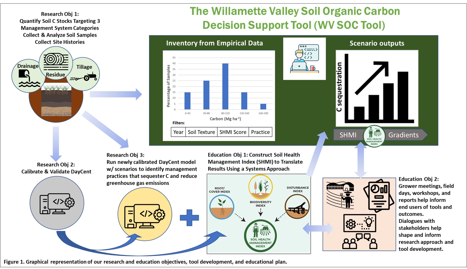
To equip farmers, crop advisors, policy makers, and conservation planners with the best science to date, we propose a combination of field soil C monitoring data and a process-based modeling effort to improve estimates of soil C dynamics in WV seed production systems. In consultation with our grower collaborators, we have identified three key management practices with potential C benefits. We will leverage and expand on previous work in the area to achieve our research goals to develop a soil C inventory for the WV grass seed industry and identification of management practices for climate mitigation and farm resiliency using both measured and modeled data (Figure 1). Our educational goals and outreach efforts will utilize multiple dissemination pathways such as field days, extension reports and manuscripts, and the WV Soil Organic Carbon Tool. This tool will host a dynamic and expandable soil C inventory that can build over time, a suite of factsheets and interpretative guides, and modeled scenario outputs to help users predict how management practices implemented on their farm may impact C sequestration and greenhouse gas emissions. Soil C workshops will be organized to provide training. Based on our findings, we aim to demonstrate the important role that Oregon seed production systems play in mitigating climate change and overall farm resilience. Initially, we will focus on C sequestration potential, but intend to build a flexible platform to include other soil health metrics over time.
Research Objectives:
- Quantify soil C stocks for the grass seed industry in the WV, OR with an emphasis on systems differing in subsurface drainage, residue, and tillage management practices.
- Calibrate and validate the DayCent model (a biogeochemical model used to predict carbon sequestration and greenhouse gas fluxes in agricultural systems) using data generated in objective 1.
- Identify which management practices support the greatest C sequestration potential using sensitivity analysis from a suite of DayCent simulations.
Education Objectives
- Translate C results into a decision support tool to help growers understand how management impacts C storage on their farms; and,
- Increase industry wide growers’ knowledge of the factors that affect soil C sequestration potential in WV grass seed systems.
Cooperators
- - Producer
- - Producer
- - Producer
- - Producer
- - Producer
- - Producer
- - Producer
Research
1.1 Tile drainage
Site Selection: The three tile drainage systems investigated included:
1) NEW Tile (fields that had subsurface tile drainage installed < 5 years (South Valley) or < 6 years (North Valley) at the time of sampling).
2) OLD Tile (fields that had tile installed 18-30 years ago (South Valley) or > 40 years ago (North Valley).
3) UNTILED (fields with no history of subsurface tile drainage).
Five fields for each tile treatment within each Valley location were identified with the assistance of David Neal (Owner of Agricultural Drainage Corporation) and Andy Gallagher (soil classifier). Within each field, three transects were geolocated during multiple scouting trips under the guidance of Mr. Andy Gallagher to ensure transects were established under the same soil type (target soil series was Dayton in the South Valley and Amity and Woodburn in the North Valley).
The target soils consist of very deep, poorly drained (Dayton), somewhat poorly drained (Amity), or moderately well-drained (Woodburn) soils that formed in glaciolaustrine deposits. Soils tend to be acidic (pH < 6.0) and are of silt loam or silty clay loam texture. They all have an apparent water table at its uppermost limit from December to April. Among the three soils, the Dayton soil tends to be considered the least productive, even with subsurface tile drainage due to a distinctive clay layer (Malpass clay), that is less receptive to drainage than other soils such as the Amity or Woodburn series https://ir.library.oregonstate.edu/downloads/5t34sj815).
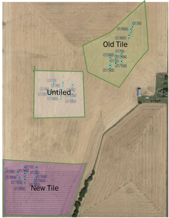
A total of 30 grass seed production fields representing 10 Old Tile, 10 NEW Tile, and 10 Untiled were identified and sampled in collaboration with five producers (two in the South Valley and three in the North Valley) (Figure 1). One of the Old Tile fields in the South Valley was not able to be sampled due to equipment failure.
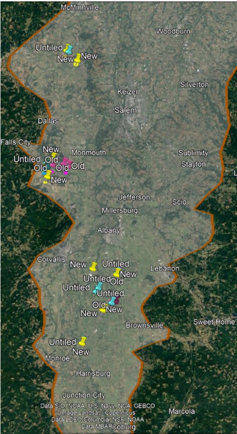
orange) with the approximate sampling locations for the three tile drainage systems (New, Old, Untiled).
Three 50-m transects were established within each targeted soil zone within each field. We sampled soil to a depth of 1 m (South Valley) and 60 cm (North Valley) at the 0 m, 25 m, and 50 m points along each transect with an ATV-mounted hydraulic soil probe (Giddings Machine Company, Inc.) and used plastic liners within a stainless-steel soil probe (4.25 cm diameter) to extract intact soil cores. The intact soil cores were removed from the stainless-steel probe, capped on either end to prevent soil loss, and placed immediately on ice packs to keep cores cool. We stored intact soil cores at 4°C immediately after returning from the field.
South Valley Sampling Campaign: Samples in the South Valley were collected in the summer of 2022. (July 21- Sept 7). A total of 126 soil cores per field were collected. Soil cores were split into three soil horizons and the 372 samples were analyzed for total soil organic carbon and nitrogen content. Additional analyses include soil bulk density which is important to convert soil C and N content (g per kg soil) to stocks (g per hectare). The rock-hard soil conditions were more than our hydraulic-powered soil coring machine could handle and ultimately sampling had to be halted to protect personnel safety (coring machine was coming disconnected from the base it was attached to and threatening to break apart) and environmental health (e.g., potential to spill hydraulic and other machine fluids).
North Valley Sampling Campaign: Samples in the North Valley were collected in the Spring 2023 (April 28-May 16). Samples were collected in the same manner as described in the North Valley except for one of the NEW tile fields where wheat had been planted. To protect the crop, samples in this field were manually collected by shovel to a depth of 30 cm and split into 0-15 and 15-30 cm increments. All other samples were collected to a depth of 60 cm. This shallower depth relative to the South Valley was selected to protect the Giddings instrumentation that had resulted in equipment failure when sampled to the deeper 100 cm depth in the previous summer.
Root Sampling:
We used the Giddings hydraulic probe to collect root cores in the same manner as that described for soil samples except root cores were extracted using a 7.62 cm diameter steel core that was 90 cm long. Relative to the soil core, the larger diameter is preferred for root sampling to optimize the quantity of roots that can be obtained. Due to the extreme soil hardness that stressed the hydraulic probe in the summer 2022 sampling campaign, we were unable to get three root cores per field. In the 2023 spring sampling campaign, the motor of the Giddings probe began failing thus, preventing the target of three cores per field as well. Despite these major challenges, our team was able to retrieve at least one core for each field. Overall, a total of 66 cores were collected with half coming from each Valley location. In the South Valley, 10 were collected in OLD, 11 in NEW, and 12 in UNTILED. In the North Valley, we collected 13 cores OLD, 9 in New, and 11 in UNTILED fields.
Soil and Root Processing:
In the South Valley, samples were split into three depths identified by genetic soil horizon due to the distinct Malpass clay layer in the Dayton soil types that can begin as shallow as 25 cm and end as deep as 74 cm. Because of the variability in the depth of the clay layer and its influence on physical and chemical characteristics of the soil, we opted to segment the soil based on horizons, instead of standardized soil depths (e.g., 0-15 cm, 15-30 cm, etc.) as this would maintain a consistent texture class across all samples. We identified the Ap/E (above the Malpass clay), Bt (Malpass clay), and BC (below the Malpass clay) horizons and recorded the depth and mass for each. Roughly, depths in the Ap/E horizon were on average 0-40cm, the Bt horizon extended to 74cm, and BC horizon 3 extended to 100cm.
The distinctive Malpass clay layer is not present in the targeted soil series in the North Valley. All soils collected from this location were separated into the standard soil depths of 0-15, 15-30, and 30-60cm.
In the lab, soil samples were separated into their respective depth increments and passed through a 4-mm sieve to homogenize the sample. A sub-sample was collected for biological assessments that require field-moist conditions as part of another project. The remaining soil was air-dried, sieved to 2mm, ground to a fine powder, and analyzed for total soil carbon and nitrogen content by combustion using a LECO CN 828 analyzer. Bulk density was calculated as the mass of the dry soil divided by volume. We measured soil pH in a 1:1 soil:water ratio and soil texture was determined by laser diffraction after isolating the sand fraction from sieving.
To simplify root processing, samples at both locations were separated into 0-15, 15-30, and 30-60 cm depths. Roots were separated from soil using a Gilson Hydropneumatic Elutriation System (aka the Rootwasher); equipment partially supported by this grant. The Rootwasher substantially decreases sample processing time, reducing labor costs and operator error. Following washing, the 198 root samples were dried at 40°C, weighed, ground, and analyzed for carbon and nitrogen content by dry combustion (LECO CN828 Analyzer).
Greenhouse gas measurements:
One of the farms in the South Valley has all three tile drainage treatments present and is otherwise managed the same (Figure 2). Annual ryegrass has been grown on this land with natural reseeding for at least three years. Sheep or cattle graze the grass in winter or spring months to manage growth and overall stand health.
In September 2022, we installed nine soil collars (20 cm diameter x 11.4 cm high) in each of the drainage areas (NEW, OLD, UNTILED). In-field carbon dioxide (CO2) and nitrous oxide (N2O) fluxes were measured with LiCor gas analyzers (Li-870 for CO2 and Li-7800 for N2O) connected to the 8200-01S Smart Chamber (Figure 3). We measured CO2 and N2O fluxes every 1-2 weeks until June 2023 when entry into the field would damage the crop and crop height and density prohibited easy passage to each collar. Fluxes were not measured for a brief period from February to March due to equipment malfunction and the need to return the equipment to the company for repair.
1.2 Residue Management
We leveraged the original residue management study as described in Trippe et al. (2021). Soil texture is an important soil physical property that influences the rate and magnitude of carbon accrual and depletion in soils. We analyzed soil texture on each sample using laser diffraction as described by Faé et al. (2019). Briefly, 5 g of soil was soaked overnight in a 1:1 v/v 10% sodium hexametaphosphate:deionized water solution (total volume 100 mL). Afterward, samples were vigorously mixed for 5 minutes, passed through a 53-µm sieve, and rinsed with deionized water to ensure all silt and clay size particles (< 53-µm) were separated from the sand particles (> 53-µm). The fraction on top of the sieve was transferred to a metal tin, dried at 60°C, and a final mass was obtained after the dried sample was completely cooled. This dry mass was identified as the sand fraction (>53-µm size fraction). Soil particles smaller than 53-µm were processed by laser diffraction using a Mastersizer 2000 (Malvern Panalytical Ltd., Malvern, United Kingdom) equipped with a Hydro 2000S. Aliquots of the remaining soil solution were dispensed into the particle size analyzer until reaching between 10–20 % obscuration. Programming for detecting particles via diffraction assumed particle density of 2.65 g cm−3, particle refractive index of 1.55, particle absorption index of 0.1, and water refractive index of 1.33. Lower limits for particle size diameter cutoffs are 6.33 μm for clay, and 56.37 μm for silt. Although the conventional diameter size for clay is < 2 μm, a larger upper limit is used to accommodate detection of elongated particles (Faé et al., 2019; Zobeck, 2004). Typically, less than 2% of the <53-μm sample was found to be greater than 56.4 μm. This small amount was added back to the sand content originally calculated by the fraction greater than 53-μm wet-sieving step. To calculate the silt and clay fractions, the mass of sand was subtracted from the original 5.0 g sample. Then the proportion of silt or clay from the laser was multiplied by this mass and divided by the total mass.
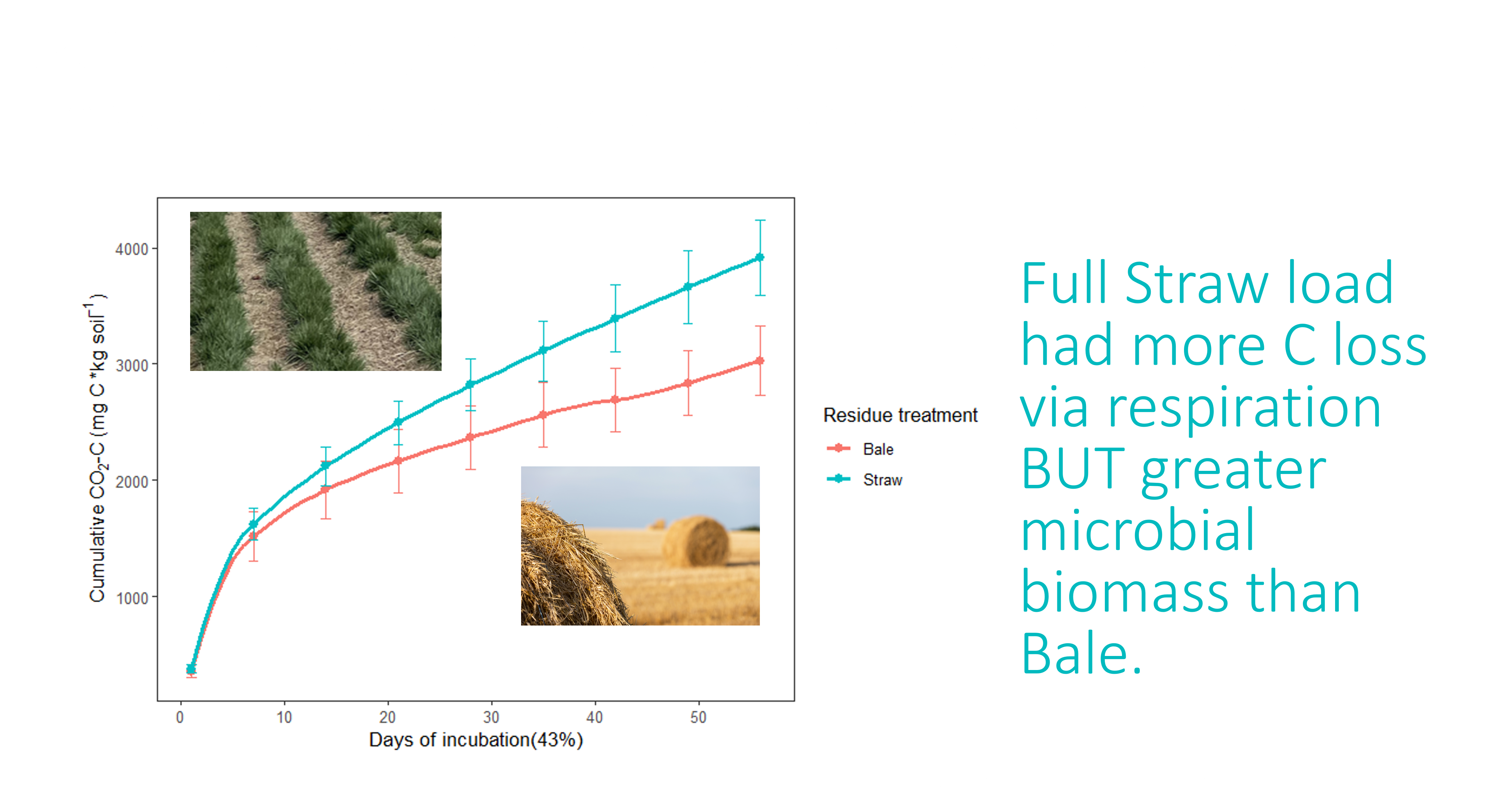
To better understand the rate of C decomposition and further control for field variability, a laboratory incubation trial was initiated. Soil samples (0-15cm) were collected in January to February 2024 from eight tall fescue (Lolium arundinaceum (Schreb.) Darbysh.) seed production fields in the Willamette Valley, Oregon. Four of these fields had been under full straw residue return (Straw), where the straw was chopped, flailed, and left to decompose in situ. In the other four fields, straw residues were baled and removed from the fields (Bale).
Tall Fescue straw residue had been collected from a representative field, dried, and ground. The carbon and nitrogen content is 46% and 0.8%, respectively.
Incubation: For each field, 40g oven-dry equivalent sub-samples were weighed into six 125-ml Wheaton serum bottles, adjusted to 43% water-holding capacity, and pre-incubated for 7 days at 25C. After the pre-incubation period, we added straw residues at a 1x or 2x rate, which is equivalent to the average 5000 lb ac-1 residue remaining following tall fescue seed harvest (extension document). A no-residue control was also included for each field sample. We used two replicates per field and treatment for a total of 144 samples (8 fields x 2 reps x 3 treatments x 3 sampling times).
We destructively sampled 1/3 of the bottles at 7 days (T1), 28 days (T2), and 91 days (T3). Weekly, set T3 was adjusted for water content, sealed with a crimp cap and septum, and incubated for 24-h at 25C. Then, CO2 subsamples were collected using a 20-ml syringe and transferred to a pre-evacuated 12-ml vial. CO2 was then measured on a Shimadzu TOC analyzer fitted with a manual gas injection port and ran in the inorganic C mode standardized with a minimum of 5 standards.
At the end of each incubation period, samples were frozen and then freeze-dried. The two lab replicates were combined, and non-decomposed straw residues were removed using a seed sorting machine. Samples were then analyzed for total soil C and N content.
1.3 Tillage Management
Site Selection: Three grower collaborators were identified who had fields under long-term (>10 year) no-till management. Each field had been under grass production and represent different management histories and soil types.
Field 1 (TF --> meadowfoam; grazing history):
- Crop history: Tall fescue system from 2013 until final harvest in 2024. System was not tilled during the 10+ years under seed production. Fescue hay following harvest was removed via baling. Prior to tall fescue, the field was planted to meadowfoam for two years and prior to that, it was under annual ryegrass production with baling of hay residue.
- Soil type: The dominant soil is Dayton series (Fine, smectitic, mesic Vertic Albaqualf). They are very deep, poorly drained soils formed in silty and clayey glaciolacustrine deposits.
- Animal integration: Cattle were grazed for approximately one month in the fall following harvest from 2013-2019.
- Tillage: in July 2024, the field received multiple (5) vertical disk passes that resulted in a soil mixing efficiency of about 25% to a depth of 4-8" depending on the pass. In September 2024, the field received lime with two shallow passes with a disk (2" deep) and a mixing efficiency of 25%. Finally, the field was lightly rolled, impacting the surface 1" to prepare the soil for planting meadowfoam in October 2024.
- Soil sampling: Baseline soil samples in the field prior to the first tillage pass were collected in July 2024. A small section of the field edge was allocated to remain in no-till conditions. This section received lime, but it was not incorporated.
- Soil amendments: Lime was applied in September 2024 with two shallow (2”) disk passes.
Field 2 (TF --> Winter Wheat--> Winter Fallow-->TF; no grazing history):
- Crop history: Tall fescue system from 2016 until final harvest in 2023. Winter wheat was no-till planted fall 2023. The field was tilled in fall 2024 and field has been fallow through the winter. Additional light tillage and herbicide applications will be done in May, prior to planting TF. The system was not tilled during the 10+ years under seed production. Fescue hay following harvest was removed via baling, but the wheat straw was incorporated.
- Soil type: The dominant soil is Amity series (Fine-silty, mixed, superactive, mesic Argiaquic Xeric Argialboll). They are very deep, somewhat poorly drained soils that formed in stratified glacio-lacustrine silts.
- Animal integration: No history of grazing.
- Tillage: October 2024 (implement details are in process).
- Soil sampling: Baseline soil samples in the field prior to the first tillage pass were collected in September 2024. A small section of the field edge was allocated to remain in no-till conditions.
Field 3 (Mixed species pasture --> winter wheat; sheep grazing history):
- Crop history: Mixed species pasture system dominated by tall fescue and chicory from 2014 until termination in 2024. System was not tilled during the 10 years. The field was not managed for seed production but served instead as pastureland for sheep.
- Soil type: The dominant soil is Willamette series (Fine-silty, mixed, superactive, mesic Pachic Ultic Argixeroll). They are very deep, well drained soils that formed in silty glaciolacustrine deposits.
- Animal integration: Annual sheep grazing from approximately September to March.
- Tillage: In October 2024 two soil disturbance events were deployed as a means to terminate the current crop: 1) a disk ripper (V-ripper) was used to a depth of 14" and a mixing efficiency of 25% and 2) vertical disk to a depth of 3" and mixing efficiency of 25%. To prepare the soil for winter wheat planting, two passes occurred. The first was a vertical disk to a depth of 4" and the second pass was a roller that helped to smooth the surface to a depth of approximately 1". Winter wheat was planted on 10.20.2024.
- Soil sampling: Baseline soil samples in the field prior to the first tillage pass were collected October 1, 2024. A small section of the field edge was allocated to remain in no-till conditions.
- Soil amendments: 80 lbs/ac of fertilizer was applied on 10/6/2024 and incorporated with a vertical disk implement.
Objectives 2 and 3: Modeling
The DayCent model is a process-based model that is used for soil C stocks changes and soil emissions of N2O and CH4 in the US national GHG inventory and reporting system (US EPA, 2019) and is the main model used in the COMET-Farm (http://comet-farm.com/) tool promoted by USDA.
The model simulates exchanges of carbon, nutrients, and trace gases among the atmosphere, soil, and plants as well as events and management practices such as fire, grazing, cultivation, and organic matter or fertilizer additions (Del Grosso et al. 2011). Soil organic matter is simulated for the top 20-cm soil layer.
DayCent includes four sub models: plant productivity, decomposition of dead plant material and soil organic matter, soil water and temperature dynamics, and N gas fluxes. The inputs necessary to use DayCent fall into four categories: (1) weather information, (2) soil information, (3) plant information, and (4) management information. There are more than 1000 parameters in the DayCent model. Although only a small subset of these is necessary for calibration, the process is labor intensive, requiring advanced computer programming skills in addition to agronomic and soil science expertise.
We were fortunate enough to leverage funding received from the OGSC that helped us secure additional funding through Western SARE (Sustainable Agriculture Research and Education) and the USDA-ARS headquarters postdoctoral research program. Through these additional sources, we have enough funding to hire a full-time postdoctoral research associate to assist with the modeling activities. We have been actively recruiting for this position for the past 9 months and have yet to find a suitable candidate. Despite this major hurdle that has substantially delayed our expected progress with the modeling steps, our CO-PI, Dr. Dan Manter, in Fort Collins, Colorado has been leading these efforts through communication with Dr. Steve Del Grosso. Dr. Manter and Dr. Moore are learning (primarily through self-taught paths) how to parameterize the model and begin some of the model runs. Over the past two months, we were able to acquire and install the model, conduct literature searches in combination with soil, root, and GHG data presented here, and have begun the calibration process for tall fescue systems in the Willamette Valley.
Update as of April 2025: We successfully identified and recruited a postdoctoral research associate who joined our team in November 2024. The research associate was onboarded and completed a week-long DayCent training course from Colorado State University Carbon Solutions Center. The training course was also completed by PIs Moore and Manter. Unfortunately, the research associate resigned after being terminated by the agency in February 2024. We are working with SARE and USDA-ARS to reallocate funds and to identify a new PhD student to complete the modeling work through Oregon State University.
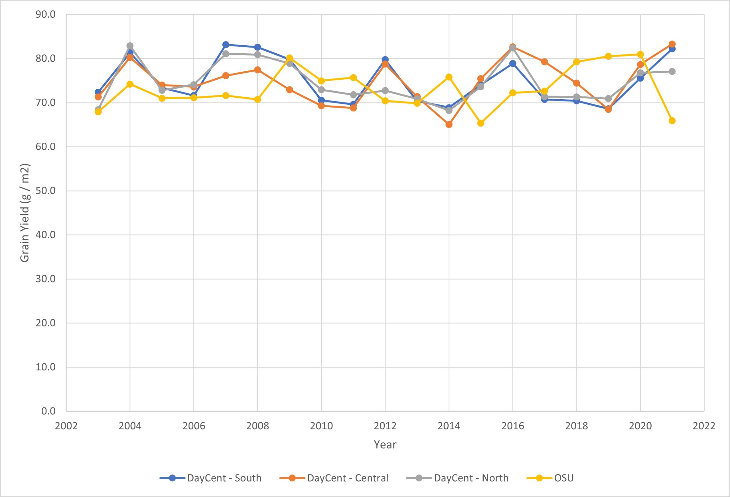
In year 1, we familiarized ourselves with DayCent v5.5.17 using one soil type and weather data from south, central, and north regions within the Willamette Valley. We modeled estimates of yield (g C in the seed m-2) with the management practices of no tile drainage, 95% straw removal, and conventional tillage for three locations in Willamette Valley (South: blue, Central: orange; North: grey). Results were in good agreement with those reported by OSU for tall fescue (yellow line) (Figure 8).
Plant productivity data files
Yield data were downloaded from OSU seed production reports from 2003-2021 (https://cropandsoil.oregonstate.edu/seed-crops/oregon-grass-and-legume-seed-production) and translated to the necessary units of g C in the seed m-2. Crop data were based on a synthesis of literature from the WV and root C data reported here.
In year 2, following our intensive week-long DayCent training, the research associate constructed regional boundaries for weather and soil data as described below. These data files better represented the acreage of seed production throughout the Valley.
Defining the acres of interest in the Willamette Valley
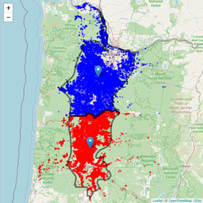
The potential boundary of relevant acres for grass seed production was determine as the intersection of the 10 Willamette Valley counties (Benton, Clackamas, Columbia, Linn, Lane, Marion, Multnomah, Polk, Washington, Yamhill) and the Willamette and Puget Sound Valleys Major Land Resource Area (MLRA 2) (Major Land Resource Area (MLRA) | Natural Resources Conservation Service). We also split the Willamette Valley into North (1,896,418 acres) and South (1,440,945 acres) sections, which followed the northern edge of Benton and Linn counties. We also identified croplands from several of the major crops in the WV from the Crop Data Layer (CDL) (https://croplandcros.scinet.usda.gov/). List crops selected from which we obtained shape files. Only cropland acres that fell within the WV portion of MLRA 2 were used for further analysis. North WV (353,678 acres) and South WV (200,151 acres).
Defining major soil series within each region of interest
SSURGO data was downloaded (R package FedData) and soil information was collected on the selected CDL polygons. Since mukey polygons may be larger than the CDL polygons, the SSURGO data was clipped to the CDL polygons. For each section of the WV, the dominant soil series (i.e., 1st element in the muname) was calculated. Each soil series could be represented by multiple munames and mukeys based on their slope or geographic position.
A unique soils.in file was created for each soil series that comprised more than 1% of the cropland area in either the North (19) or South (25) WV (Soil acres summary table). SSURGO data (reported by genetic horizons) was split into the following layers (0-2, 2-5, 5-10, 10-20, 30-45, 45-60, 60-75, 75-90, 90-105, 104-120, and 120-150 cm). For shallow soils, any missing data at the deeper depths, was assumed to be the same as the lowest soil horizon value reported. Final values were calculated as the weighted mean across all mukeys for that soil series using acres as the weights.
Defining weather data files within each region of interest
Weather data at the centroid of each of the North and South WV polygons were downloaded from DayMet (https://daymet.ornl.gov/) using daymetR.
1.1 Tile drainage management results:
A total of 774 soil samples were analyzed for total soil C and N content, bulk density, texture, and pH. This total is comprised of 378 soil samples from the South Valley (14 fields x 3 transects x 3 points x 3 depths) and 396 samples from the NorthValley [(14 fields x3 transects x 3 points x 3 depths) + (1 field x3 transects x 3 points x 2 depths)].
The results from the South Valley were part of another project and have been reported previously (Breza et al., 2022). Overall, soil C stocks were not significantly different between tile drainage systems and averaged 78.4 Mg C ha-1 (approximately 35 tons ac-1) to a depth of 100 cm.
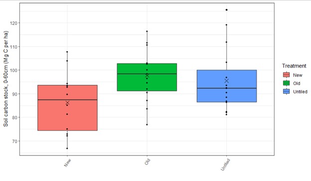
The mean soil carbon stock across all fields in the North Valley was 93.4 Mg C ha-1 (approximately 42 tons ac-1) to a depth of 60 cm. There was no statistically significant difference in soil carbon stocks between tile drainage treatments. High field-to-field variability (> 40 Mg C ha-1 within each treatment), likely the result of crop rotations histories and plant species grown at the time of sampling, which can influence the amount and turnover of carbon in the soil, limited our ability to find statistically significant differences. However, certain trends did exist. For example, over the entire 60 cm profile, NEW had the lowest soil C stocks (86.2 Mg C ha-1) and OLD had the highest soil C stocks (97.7 Mg ha-1) (Figure 2).
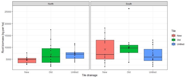
Viewing soil C stocks at each depth increment (Figure 3), UNTILED was greatest at the surface (0-15 cm). Prolonged saturated conditions can decrease organic matter decomposition rates and result in carbon accrual, which may explain this observation. Deeper in the soil profile, OLD soil C stocks tend to increase relative to C stocks in UNTILED and NEW. These trends suggest that soil C may initially be depleted following installation of tile drainage within the first 5-6 years. However, over time, root growth may compensate for the depletion, replenishing soil C at depth. Our root biomass followed this similar pattern (Figure 4) with lower biomass in NEW compared to OLD (South Valley panel in Figure 4), further supporting this concept. Thus, it is difficult to definitively conclude that tile drainage had no effect on soil C sequestration. Rather it may be a function of time since drainage installation, with the degree of soil C depletion (e.g., NEW) and accrual (e.g., OLD) possibly related to the crops grown in each system.
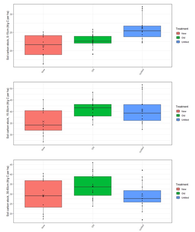
Within the 0-15 cm depth, we estimated soil C stocks of 23,318 kg C ha-1 for the North Valley fields, which are on the lower end but similar to those reported by Griffith et al. (2009). Our data to 60 cm in the North Valley and 100 cm in the South Valley are among the first to report carbon stocks beyond the surface and are the first to our knowledge, to report specifically in tile-drained fields.
Comparing soil C stocks from 0-30 cm in the WV grass seed production systems to national cropland averages (0-20 cm), WV seed averages in this study are about 28 tons /ac whereas US cropland averages about 20 t/ac (Guo et al., 2006). Normalizing our 30 cm depth to 20 cm, results in an estimated 18.6 tons per acre in these WV soils. These values are slightly lower than those reported in other studies in the valley and are possibly related to our targeted soils which tend to have lower productivity ratings than other soils common in the valley.
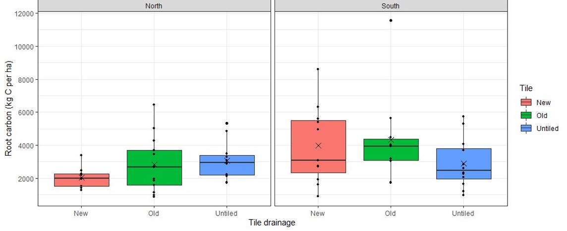
No significant differences were observed with root biomass or root C stock. In general, average root biomass (Figure 4) and root C stock (Figure 5) were lowest in NEW for the North Valley. On average, roots contained approximately 43% carbon, which is slightly higher than that reported by Chastain (n.d.).
Greenhouse gas emissions
Greenhouse gas emissions were measured in a single field in the South Valley where all three tile drainage systems were present (Figure 6). Cumulative soil respiration (CO2-C flux) is a measure of root and microbial respiration from the soil. CO2-C flux was statistically greater in OLD (12.3 Mg CO2-C ha-1) than in NEW (10.3 Mg CO2-C ha-1) or UNTILED (10.4 Mg CO2-C ha-1). This may be attributed to greater root biomass observed in OLD (average of 5748 kg ha-1) compared to NEW (1803 kg ha-1) or UNTILED (3374 kg ha-1) (Note: these data are from the single South Valley field unique to the GHG measurement study). Root biomass results were not significantly affected by tile drainage system. Unfortunately, the equipment failure when collecting root cores during the very dry months in summer 2022, resulted in insufficient data points to fully evaluate this hypothesis. However, the trends of greater root biomass in OLD compared to the other treatments warrant further investigation.
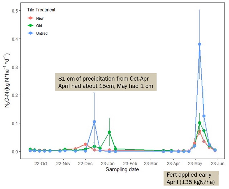
N2O is an important GHG with approximately 272 times the global warming potential of CO2. Agriculture is a leading contributor to national N2O emissions resulting from losses during nitrogen fertilization, manure applications, and rice cultivation. N2O can be formed under anaerobic conditions during denitrification or under more aerobic conditions during nitrification following nitrogen fertilization. When O2 is limiting denitrification can more easily go to completion and form N2. This pathway is preferred because N2 is an inert gas, making up nearly 80% of our atmosphere. During the transition periods from complete saturation (and absence of O2) to field moist or drier conditions, microbes tend to produce more N2O relative to N2. In general, N2O tends to be produced when 50-70% of soil pores are filled with water (referred to as water-filled pore space).
During the winter months of our 2022-2023 sampling period, we measured relatively low N2O fluxes (Figure 7). Approximately 81 cm of precipitation fell in the area from October 2022 to April 2023. Saturated conditions resulting from the high rainfall would create saturated soil conditions even in the areas where tile drainage is present. This factor along with cool temperatures and presumably low residual nitrate-N likely is assumed to have resulted in complete denitrification (i.e., production of N2 relative to N2O). However, soils dry down relatively rapidly following the cessation of
rains in late spring (late April/early May in 2023). Additionally, soils are warming, stimulating soil microbes and N fertilization occurs (early April 2023). The combination of these factors results in the majority of N2O production during a 4–6-week period from May to June. During this period, UNTILED areas have the greatest N2O flux and rates remain higher for longer than OLD and NEW tile areas.
In the 2023-2024 sampling period, our initial flux measurements (October-November 2023) revealed similarly low N2O fluxes as were measured in 2022 (Figure 8). Approximately 81 cm of precipitation fell in the area from October 2022 to April 2023. Saturated conditions resulting from the high rainfall would create saturated soil conditions even in the areas where tile drainage is present. This factor along with cool temperatures and presumably low residual nitrate-N likely is assumed to have resulted in complete denitrification (i.e., production of N2 relative to N2O). However, soils dry down relatively rapidly following the cessation of rains in late spring (late April/early May in 2023). Additionally, soils are warming, stimulating soil microbes and N fertilization occurs (early April 2023). The combination of these factors results in the majority of N2O production during a 4–6-week period from May to June. During this period, UNTILED areas have the greatest N2O flux and rates remain higher for longer than OLD and NEW tile areas.
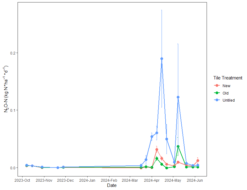
Greater fluxes in UNTILED could be related to longer dry down period throughout the soil profile, leading to ideal soil moisture and O2 conditions for N2O production (i.e., between 50-70% water-filled pore space). When we zoom in on this period and evaluated the water-filled pore space measured in top 10 cm (4 in), we observe that UNTILED remained in the optimal water-filled pore space range for a longer time than OLD and NEW tile areas. For example, on April 30th, UNTILED had approximately 70% water-filled pore space, whereas OLD and NEW were between 50-60%. On May 13h, UNTILED remained high at approximately 60%, whereas OLD and NEW were below 40% water-filled pore space. By May 20th all fields were below 20% water-filled pore space where N2O production is essentially zero (Figure 8).
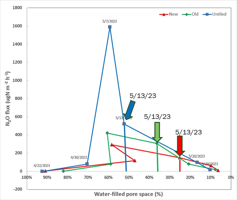
Cumulative N2O flux initially was greater in OLD than NEW or UNTILED during early spring weeks, but by the end of the sampling period, UNTILED had the greatest cumulative flux of 4.75 kg N2O-N ha-1. Although not significant, the ranking of cumulative flux was UNTILED > OLD (3.18 kg N2O-N ha-1) > NEW (1.97 kg N2O-N ha-1). Overall, these values tend to be lower than those reported in mid-western cropping systems under tile drainage.
1.2 Residue Management and Soil Texture
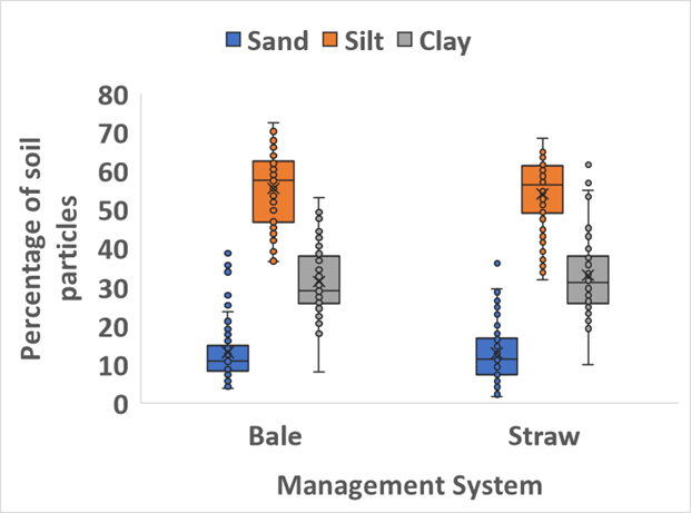
All samples have been analyzed for soil particle size analysis, which is expressed as the percentage of clay, silt, and sand particles in the soil sample. On average, fields contained 30.5% clay, 56.9% silt, and 12.6% sand in the 0-30cm, and 34.2% clay, 52.6% silt, and 13.2% sand in the 30-100cm depth. Most soils were classified as silty clay loams or silty clays (Figure 1). Of note is the variability across fields (Figure 1.2.1; Table 1.2.1). This is important because there is a strong relationship between clay content and soil carbon content that is independent of management (Figure 1.2.2).
Table 1.2.1. Summary of soil clay, silt, and sand content (%) for the 0-30 and 30-100 cm depths
|
|
Clay |
Silt |
Sand |
|
0-30 cm depth |
(%) |
||
|
Overall average |
30.5 |
56.9 |
12.6 |
|
Minimum field average |
21.2 |
39.3 |
4.9 |
|
Maximum field average |
55.8 |
68.4 |
27.8 |
|
30-100 cm depth |
|
|
|
|
Overall average |
34.2 |
52.6 |
13.2 |
|
Minimum field average |
19.7 |
35.4 |
3.2 |
|
Maximum field average |
59.7 |
66.9 |
32.9 |
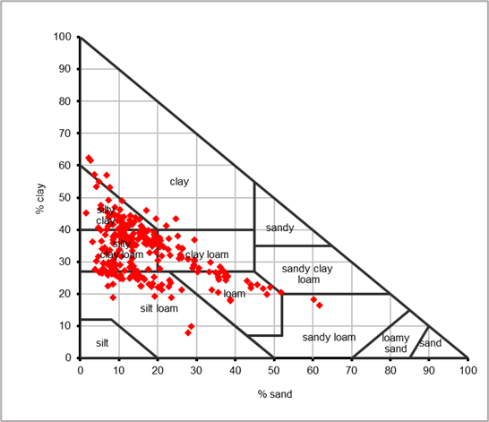
Figure 1.2.1. Plot showing the distribution of textural classes in both depths for the residue management samples (N = 144).

When we retested for the effect of management (baled vs full straw) using clay content as a covariate, we reduced the variability (described in a statistical term, “standard error”) by approximately 1.2 Mg C ha-1 for each comparison (Table 2). The effect of management remained statistically insignificant, but model statistics were improved (i.e., the test statistic values increased, and p-values decreased) indicating the importance of including clay content in the model. Despite improvement to our analysis with the inclusion of clay, we feel that field-to-field variability continues to hinder our ability to confidently assess whether residue management impacts soil carbon sequestration potential. Accounting for other co-factors (e.g., tillage history, crop rotation history, etc.) may help to further reduce the variability not related to the effect of residue management. Soil sampling for this study was conducted based on soil maps, which are intended to be used as guides, and the mapped unit may not always be what is present on the ground. This is one reason our follow-up study on tile drainage was constrained to the same/similar soil types. The sampling for that study was done following the expert guidance of Mr. Gallagher, who is a certified soil classifier. In the residue study described here, the dominant soil type was targeted on each field but different soil types within and between fields can vary in their productivity and drainage classifications; properties known to influence crop growth and thus, soil carbon storage potential. Our team is working with statisticians to determine if we can account for these differences using advanced statistical tools.
Table 2. Summary of mean soil carbon stocks (Mg ha-1), standard error, and lower and upper confidence limits with and without the inclusion of clay in the model.
|
Model |
Management |
Mean
|
Standard error |
Lower confidence limit |
Upper confidence limit |
|
|
|
(Mg ha-1) |
|||
|
With clay |
Bale |
84.1 |
4.33 |
75.2 |
93.1 |
|
Straw |
91.2 |
3.98 |
82.9 |
99.4 |
|
|
Without clay |
Bale |
83.8 |
5.61 |
72.2 |
95.5 |
|
Straw |
91.4 |
5.16 |
80.7 |
102.1 |
|
Residue incubation results:
Objectives 2 and 3: Modeling
One of the first steps in calibration is to align crop productivity and grain yield with known values. Modeled estimates of yield (g C in the seed m-2) with the management practices of no tile drainage, 95% straw removal, and conventional tillage for three locations in Willamette Valley (South: blue, Central: orange; North: grey) were in good agreement with those reported by OSU for tall fescue (yellow line) (Figure 8). The results to date also show a good agreement between publicly available plant productivity data (above- and below-ground biomass) and DayCent estimates (data not shown). More detailed calibration efforts for soil properties (soil C and N) using the data collected in 774 soil samples collected in Objective 1 are on-going. This data will be critical for calibrating the soil component of the DayCent-CABBI model under differing climates, soil series, and management histories for grass seed production across the Willamette Valley.
Research Outcomes
Understanding C cycling dynamics in the Willamette Valley will help us determine how local agricultural management can aid in C sequestration under a changing climate. This is the first step to survey and quantify soil C stocks and GHG emissions in tile drainage sites. Our results suggest that soil C storage is substantial in these grass seed production systems storing between 78 to 94 Mg C ha-1 in the South and North Valley fields, respectively. Based on our preliminary assessment, long-term tile drainage does not negatively affect soil carbon and has a positive effect on GHG emissions relative to fields left untiled.
We will continue to actively recruit the necessary postdoctoral associate to complete the modeling expertise for this project.
As part of a larger soil carbon and soil health assessment effort, we are in the final stages of synthesizing and interpreting our results for the tile drainage projects. In addition to a suite of soil health indicators, soil texture is the final step relevant to this study that is 75% complete on the nearly 800 soil samples collected. Soil texture is an important variable as finer texture soils (e.g., more silt and clay content relative to sand) are associated with more C regardless of management. Once complete, these data may aid in reducing some of the field‐to‐field variability, improving interpretation.
Finally, we will translate the results reported here into 1‐2 submissions to the annual Seed Research Report published by OSU Crop and Soil Science Department.
Education and Outreach
Participation Summary:
Education Objectives and Analyses
- Translate C results into a decision support tool to help growers understand how management impacts C storage on their farms; and,
- The Soil Health Management Index integrates all the soil health principles and is the compilation of three independent indices that can also be used individually to address discrete management questions related to soil health and C sequestration potential. The three indices are the biodiversity index, the disturbance index, and the root/cover index. An independent rating will be generated for each based on a 10-year rotation and include crops, tillage, and animal integration.
- Increase industry-wide growers’ knowledge of the factors that affect soil C sequestration potential in WV grass seed systems.
- In year one, we scheduled meetings with farmers, presented preliminary results at farmer-focused and student-focused venues and conducted a survey.
- In year two, we continued our collaborative meetings with farmers, developed a soil health factsheet, further refined and built an online beta-version of the Soil Health Management Index, and presented preliminary results at farmer and industry focused events.
As part of the development of the Soil Health Management Index (SHMI), we have met informally with our farmer cooperators as well as OSU extension staff to obtain information to help build the disturbance index. We are using the STIR rating system as described above and need more details about tillage depth, speed used with the implements, and the different implements commonly used in seed production. The crop rotation cycle and inclusion of livestock as part of the biodiversity index are also being discussed to determine the most appropriate cycle length, crops used, and numbers and duration of grazing animals.
2024 Education and outreach activities
Our outreach and education activities so far have included educational presentations at extension events to share the findings of the project so far.
We met with individual growers to gather field history information while refining the questionnaire used together information to calculate the Soil Health Management Index. In addition, a soil health fact sheet was developed and published.
2024 OSU Extension seed and cereal crop production meetings:
Dr. Moore gave a presentation at a series of fall Extension meetings in 2024. She introduced the project and shared preliminary data related to greenhouse gas emissions in fields with and without tile drainage. Real-time polling during the presentation was used to collect information about attendees’ typical management practices as well as attitudes toward soil health. These half-day meetings were held in Salem, Tangent and Forest Grove, Oregon on September 13 and 14, 2023. There were 182 attendees who included growers, field agronomists, and other industry professionals. We received 67 responses to the survey questions.
The questions and responses by the participants are included below and separated by location. Tangent, OR is considered South Valley; Salem, OR is Mid/Central Valley; and Forest Grove is North Valley.
|
Question 1. Please select the grass seed crop that is the dominant crop for your farm. The following questions will be based on this selection. |
||||
|
Answer |
Tangent |
Salem |
Forest Grove |
Total |
|
Annual ryegrass |
32% |
3% |
0% |
12% |
|
Perennial ryegrass |
9% |
25% |
7% |
16% |
|
Tall Fescue |
50% |
53% |
87% |
59% |
|
Fine Fescue |
0% |
9% |
0% |
4% |
|
Orchard Grass |
0% |
3% |
0% |
1% |
|
NA |
9% |
6% |
7% |
7% |
|
Response count |
22 |
32 |
15 |
69 |
|
Question 2. Consider all acres for your selected crop. Do you bale the straw or chop and flail? |
||||
|
Answer |
Tangent |
Salem |
Forest Grove |
Total |
|
All or almost all baled (>90% baled) |
28% |
70% |
38% |
51% |
|
Mostly baled (60-90% baled) |
56% |
15% |
38% |
31% |
|
About half and half (40-60% baled) |
11% |
3% |
13% |
7% |
|
Mostly chop and flail (60-90% chopped) |
0% |
3% |
0% |
1% |
|
All or almost all chop and flail (>90% chopped) |
6% |
9% |
13% |
9% |
|
Response count |
18 |
33 |
16 |
67 |
|
Question 3. Based on the crop selected, what percentage of ground do you till on an annual basis? |
||||
|
Answer |
Tangent |
Salem |
Forest Grove |
Total |
|
<10% |
6% |
16% |
6% |
11% |
|
11-30% |
47% |
63% |
75% |
62% |
|
31-50% |
29% |
13% |
13% |
17% |
|
51-70% |
6% |
0% |
6% |
3% |
|
71-90% |
6% |
3% |
0% |
3% |
|
>90% |
6% |
6% |
0% |
5% |
|
Response count |
17 |
32 |
16 |
65 |
|
Question 4. For your selected dominant crop, consider a 10-year crop rotation cycle, how many different crops will you grow? |
||||
|
Answer |
Tangent |
Salem |
Forest Grove |
Total |
|
1 |
0% |
0% |
0% |
0% |
|
1-2 |
33% |
18% |
13% |
21% |
|
2-4 |
61% |
73% |
81% |
72% |
|
5+ |
6% |
9% |
6% |
7% |
|
Response count |
18 |
33 |
16 |
67 |
|
Question 5. When making management decisions on my farm, soil health/C sequestration is: |
||||
|
Answer |
Tangent |
Salem |
Forest Grove |
Total |
|
Very important |
22% |
17% |
25% |
21% |
|
Somewhat important |
39% |
39% |
50% |
42% |
|
Neutral |
17% |
11% |
25% |
17% |
|
Somewhat unimportant |
11% |
17% |
0% |
10% |
|
Not important at all |
11% |
6% |
0% |
6% |
|
I’m not really sure what soil health is but I’d like to learn more! |
0% |
11% |
0% |
4% |
|
Response count |
18 |
18 |
16 |
52 |
2024 Virtual Coffee Hour
Dr. Tanner holds a monthly virtual Coffee Hour program where information about ongoing research projects is shared with field crop producers, agronomists and other industry professionals. Dr. Lauren Breza presented results from a study of how tile drainage influences soil carbon in local seed production systems on November 14, 2023. These data are being included in the modeling and decision support tool efforts. There were 19 attendees, and 4 views of the recorded presentation.
2024 Cooperator meeting
Drs. Moore, Trippe, and Tanner met with six grower cooperators on the project on March 6, 2024. Drs. Moore and Trippe presented an overview of the findings of this project so far. We then led a guided discussion about several aspects of the project. The discussion included considerations and priorities for data collection related to the impact of occasional tillage. The growers helped clarify the situations where this practice is most likely to occur. We also discussed the soil health management index (SHMI) that we are developing. The growers shared how they might use this tool on their farm and provided feedback on our plans. We will use information gathered in this conversation to design how growers will enter information into the SHMI tool.
2025 Education and Outreach Activities
2025 OSU Extension seed and cereal crop production meetings:
Dr. Moore gave presentations at a series of three Extension meetings. She discussed soil carbon storage in soils, and the unique characteristics of grass seed production systems that influence soil carbon storage. The presentation also included research findings from studies on straw decomposition in grass seed fields. These half-day meetings were held in Salem, Albany and Forest Grove, Oregon on January 7 and 8, 2025. There were 249 attendees who included growers, field agronomists, and other industry professionals.
2025 Presentations at industry meetings:
Dr. Moore gave a presentation at the Oregon Seed Growers’ league annual meeting on December 9, 2024. The Oregon Seed Growers League is a grower led organization, and their annual meeting attracts more than 400 attendees each year. A poster presentation about the Soil Health Management Index was presented at the Oregon Ryegrass Growers’ Association Annual Meeting on January 15, 2025. There were 175 attendees at the 2025 Oregon Ryegrass Growers’ Association Meeting.
Soil Health Management Index (SHMI) questionnaire refinement:
The SHMI decision support tool will require growers to enter detailed management history for their farms. Farmers are much more likely to use the tool if the data entry process is easy to understand and use. After developing the questionnaire, we met with five cooperating growers and walked them through the questionnaire and asked for their feedback. This process helped refine the way questions were phrased, while gathering management history for fields used in the study.
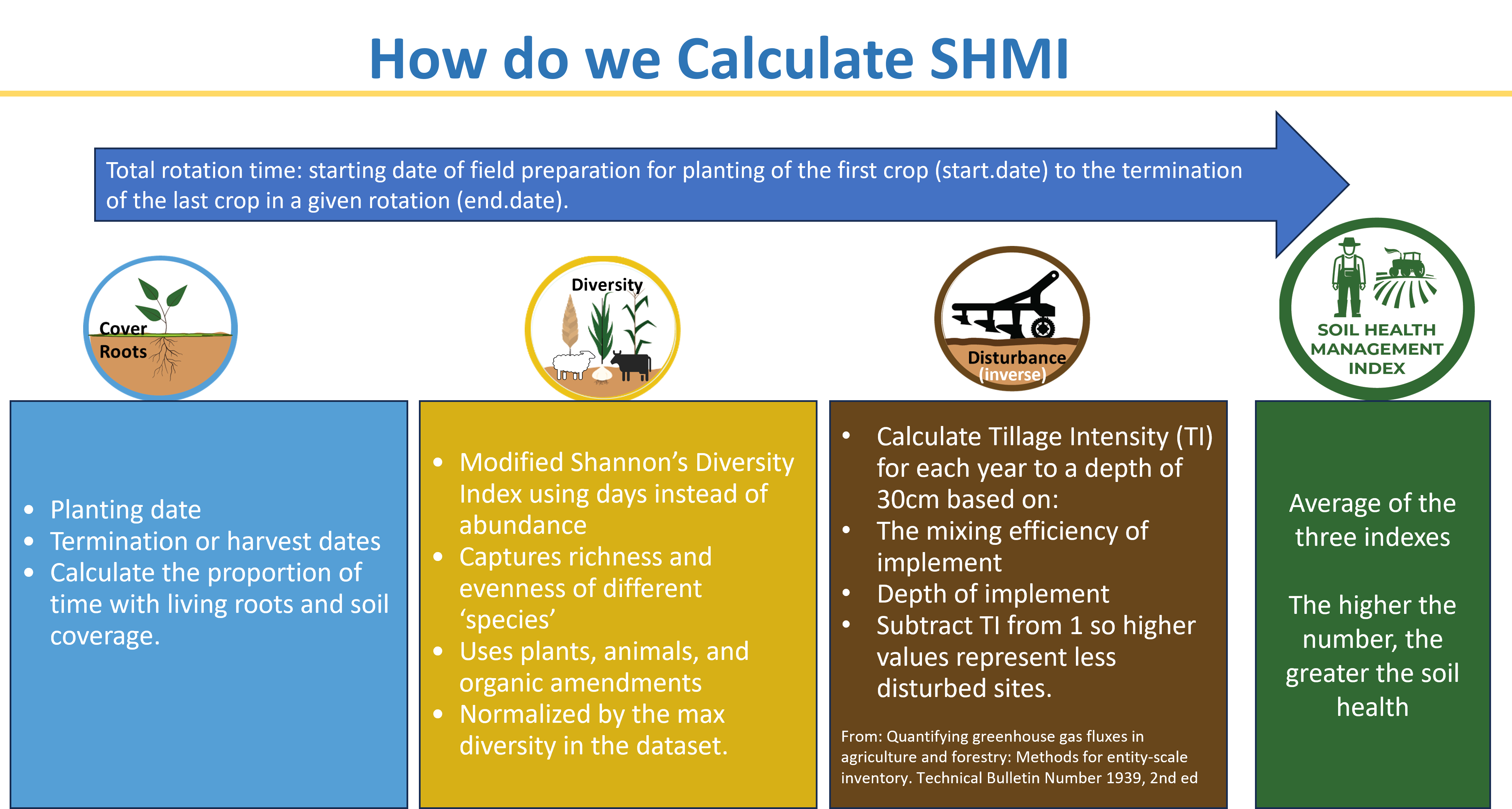
Soil Health Management Index (SHMI) calculation: The first step is to identify an appropriate length of time. Our current version uses the total rotation time which begins with field preparation of the first crop in a rotation and continues until the last crop in that rotation is harvested or terminated. The length of this time is dependent on the type of system. A corn-soybean rotation would therefore be 2 years whereas a wheat, pea, fallow, oat would need 4 years to complete the full rotation.
We then developed independent algorithms to calculate a soil health cover/roots index, a biodiversity index, and a soil disturbance index (Figure below). To calculate the Cover/Roots subindex we calculate the proportion of time with living roots and soil coverage using the planting and termination dates of each crop. For the biodiversity index, we use a modified Shannons diversity index using days instead of abundance. This index captures richness and evenness of different ‘species’ and extends beyond the traditional definition of 'species' and uses the plants, animals, and any organic amendments (e.g., manure, compost, etc). This value will be normalized by the maximum diversity in the dataset. The disturbance index is calculated with only tillage information. We have opted to use the tillage intensity formula used by the EPA inventory for GHG fluxes which is the same calculation used in the SWAT model. It is based on the mixing efficiency and depth of each tillage implement used to a depth of 30 cm. The value is from 0-1 and we subtract it from 1 so that higher values represent less disturbed sites. Lastly, we average these three subindexes to obtain an overall SHMI score. For each subindex and the overall score, the higher the number the greater the soil health.
Soil health fact sheet:
We leveraged our SARE funding and secured supplemental funding to create a factsheet, titled “Grass Seed Crops – Stewarding the Land by Sustaining the Soils” was developed by Drs. Trippe and Moore. The publication was supported with additional funds provided by the Oregon Grass Seed Councils and is hosted on the Oregon Seed Council's website. Eventually we intend on populating the inventory and SHMI tool with this and other factsheets on soil carbon and soil health in grass seed production systems.
GRASS SEED CROPS STEWARDING THE LAND BY SUSTAINING THE SOILS
Next steps
We have planned a half day workshop on soil carbon and soil carbon markets on February 19, 2025 in Albany Oregon. The agenda for the workshop includes:
- An overview of soil carbon cycling by Drs. Moore and Trippe.
- A presentation by Dr. Tanner on farming practices for grass seed production and how they influence soil carbon.
- An overview of local and regional NRCS cost share programs for soil health by Nick Sirovatka, NRCS Regional Soil Health Specialist.
- Keynote presentations by Dr. Lauren Gifford on soil carbon markets, how they are structured and barriers to participation for farmers.
- A guided audience discussion.
We have drafted a second factsheet, "Incentivizing Soil Health in Seed Production -A Guide to Carbon Markets and Conservation Programs." This draft is currently under review by the public relations subcommittee of the Oregon Seed Council and the USDA leadership for approval for publication. Once approved, we intend to host this factsheet on the OSC's website along with our first factsheet on Soil health and stewardship in grass seed production systems (described above).
Education and Outreach Outcomes
- Carbon sequestration
- Soil health
- Greenhouse gas emissions