Final report for GNE20-233
Project Information
Crop damage is a persistent issue faced by farmers nationwide, resulting in staggering costs to farmers in crop loss. Ungulate species such as white-tailed deer (Odocoileus virginianus) and sika deer (Cervus nippon) are a major source of agricultural damage through extensive browsing. Often a farmer’s only solution to mitigate browsing losses is through crop damage permits to hunt deer on their farm. However, deer populations occur over larger scales than a single property, limiting farmers’ abilities to actually reduce local deer densities through hunting and leaving them ineffective in reducing crop damage by ungulates. Surrounding habitats can reduce or exacerbate impacts on crop damage – reducing damage by providing additional food that lowers the intensity of deer browsing on crops or exacerbating damage by providing refuge to deer that actively browse on agricultural fields. My research looks to examine the effect that adjacent habitat composition and configuration has on crop damage. Our research approach was two-fold: utilize high-resolution dietary analysis using metabarcoding plant DNA present in ungulate fecal pellets allows crop damage to be quantified as well as quantifying crop damage present in the agricultural field through crop damage surveys. Then through combining these results with landscape level metrics of the surrounding habitats to reveal how habitats in close proximity to agriculture influence crop damage. Our inability to successfully amplify and sequence plant DNA in the collected fecal pellets was an unexpected challenge, that forced us to pivot and focus primarily on our second approach in quantify crop damage occurring in the agricultural fields. We found that crop damage occurs heterogeneously across the entire agricultural field, but the most intense depredation occurs in the corners and edges of the fields. Crop damage decreases as distance to the edge of the field increases but edge land uses play a significant role in influencing the intensity of damage. Edges comprising CRP, forest, and marsh had higher levels of damage compared to agricultural and developed edges. When looking at how the broader landscape influences crop damage we found that as core area and number of patches present in the landscape increased so did crop damage, indicating that landscape fragmentation intensifies crop damage in the surrounding agricultural fields. We also found that CRP and forest were the most influential land use types present in the landscape. As forest mean area increased and forest connectivity decreased, crop damage increased. The opposite relationship was present for CRP, as mean area decreases, and connectivity increases, crop damage increased. Larger less connected forested patches and smaller more connected CRP patches present in the landscape increases the intensity of crop damage. Lastly, we found that deer browse pressure influences crop yield. As the browse pressure increases, the yields declined, and this relationship was present across the entire field. This research provides evidence that farmers have options beyond trying to reduce local deer densities to mitigate crop damage. Through reducing edge types that result in increased browse pressure, reducing overall landscape fragmentation on their farms, and reducing large, less-connected forested patches and smaller more connected CRP patches can help to mitigate the impacts of crop damage.
The specific objectives of this research are to:
(1) Determine the impact that the composition and configuration of neighboring habitats (forests, marshes, fallow fields) within agricultural landscapes have on the proportion of agricultural crops in a deer’s diet.
Hypothesis 1: Overall area, number of patches and connectivity of neighboring habitats will decrease the proportion of agricultural species present in the diet of the deer.
Hypothesis 2: The proportion of agricultural species present in the diet of the deer can be explained by the composition and configuration of neighboring habitats.
Hypothesis 3: Reliance on plant species present in neighboring habitats will vary through time depending upon the abundance and availability of crops.
(2) Evaluate the impact of dietary niche overlap of sympatric deer species has on crop damage.
Hypothesis 1: We will observe higher overall deer densities in regions where both deer species occur than regions where just white-tailed deer or sika deer occur in isolation.
Hypothesis 2: Agricultural species will make up a smaller proportion of the diet of white-tailed deer and sika deer in regions where they co-occur due to interspecific competition for crop resources.
Hypothesis 3: Despite lower per capita crop consumption, crop damage will be greater in areas where the species co-occur due to higher densities.
Hypothesis 4: Higher deer densities will be supported by a greater reliance on plant species from neighboring habitats, and we expect to see a wider dietary breadth in regions where both species co-occur.
* Objective 2 had to be modified due to restricted access to farms in regions which both species co-occur. COVID-19 limited our ability to interact with farmers in these regions as well as farms that were possible site locations being sold to new owners that did not want to participate in our study. We were only able to gain access to two farm sites in which both species co-occur resulting in not a large enough sample size to proceed with this objective. I instead reallocated this effort to pursue a related question on the spatial distribution of crop damage at the patch and landscape-level. Objective 3 below outlines this new line of enquiry.
(3) Understand landscape and patch dynamics that influence the spatial distribution of crop damage at the patch and landscape-level
Hypothesis 1: Edge habitat composition will influence the prevalence and overall distance crop damage occurs into the agricultural field (patch-level).
Hypothesis 2: Field configuration will impact the level of crop damage occurring within the agricultural field (patch-level).
Hypothesis 3: Composition and configuration of neighboring habitats will influence the proportion of crop damage the entire agricultural field experiences (landscape-level).
Hypothesis 4: Neighboring habitats not directly adjacent but interconnected to the agricultural field will impact the proportion of damage the entire agricultural field experiences (landscape-level).
Hypothesis 5: Higher proportions of agriculture in the landscape will result in lower levels of crop damage across the entire agricultural field (landscape-level).
The purpose of this project is to examine the effect that landscape configuration and composition of surrounding habitat types has on crop damage by deer. Crop damage is a persistent issue faced by farmers nationwide; surveys have shown that crop damage inflicted by deer is the most widespread form of wildlife damage to crops (Conover and Decker 2018; Wywialowsky 1994, Conover 1998). Ungulates, specifically white-tailed deer (Odocoileus virginanus) and sika deer (Cervus nippon), damage crops through browsing and are a major source of agricultural damage, both of which occur on the Eastern Shore of Maryland (Claslick and Decker 1979, Conover 2001, Conover and Decker 2018, DeVault et al. 2007, Springer et al. 2013). Often a farmer’s only solution to mitigate crop damage is through crop damage permits that allow the increased harvest of deer on their farms. However, culling deer on-site may not solve the problem, as deer populations occur at larger scales than a single property. Although crop damage by deer often correlates with deer population density, not all deer present in an agricultural landscape consume the same proportion of agricultural species (Bleier et al. 2012). Agricultural fields do not occur in isolation but are surrounded by a complex matrix of habitats. Deer frequently utilize habitats surrounding agricultural fields. How do surrounding habitats affect deer consumption of crops? Surrounding habitats have been suggested to negatively and positively impact the amount of crop damage occurring on the adjacent fields. Deer can forage on plant species present in habitats surrounding agricultural fields mitigating deer browsing on crops, or deer can utilize these habitats as refuge resulting in increased deer densities and increased browsing pressure on crops. However, no research to date has tried to directly quantify how surrounding habitats mitigate or intensify crop damage.
My research quantified crop damage inflicted by white-tailed deer through conducting damage surveys across agricultural fields. Through combining the damage inflicted on agricultural fields with landscape metrics such as patch size, patch density, and patch connectivity of adjacent habitats, we were able to better understand how neighboring habitats to agriculture influence crop damage. Data on how adjacent habitats influence crop damage resulted in alternative management recommendations to mitigate crop damage for farmers and stakeholders than mitigating local deer populations. As many agricultural landowners in my study region own adjacent habitats as well as their agricultural fields, the opportunity for implementing deer management in adjacent habitats is a useful alternative. Strategic community partners have helped me to develop recommendations for best practices based on my findings and disseminate these results to landowners beyond the few sites where the research was conducted.
Cooperators
Research
The following objectives will be accomplished via field experiments established in Dorchester, Wicomico, Worcester, and Somerset Counties, Maryland and lab work conducted at George Washington University.
Objective 1. Evaluate the impact that the configuration and composition of adjacent habitats to agricultural fields in the landscape have on crop damage.
In order to investigate how varying composition and configurations of adjacent habitats influence crop damage, fecal pellets were collected across farms in order to be analyzed for dietary profiles. Fecal pellets were collected randomly throughout the predominant habitats in the landscape (agricultural fields, forested regions, and marshes). Time-based fecal pellet accumulation curves were utilized to ensure an exhaustive search. The number of fecal pellets discovered were graphed by the time spent collecting these fecal pellets, making sure that the number of new fecal pellets discovered asymptotes indicating overall fecal abundance. This indicated the sampling effort was adequate to collect all fecal pellets present. Fecal pellets were collected during 3 time points throughout the year in order to understand the seasonal variation in the importance of neighboring habitat. Collections occurred in March prior to planting, June during the growing season of the crops, and lastly September-October prior to harvest.
Fecal pellets were visually inspected for freshness based on pellet color, consistency, and sheen (Brinkman et al. 2010). Fecal pellets were ranked for freshness ranging from high quality (sticky with mucus, slight sheen on pellets, soft texture) to low quality (firm and dry but still with a sheen of mucus) (Kalb and Bowman 2018). We did not count fecal pellets that show signs of mold, appear broken or decayed, or lack a mucosal sheen on the exterior. A GPS unit was utilized to collect exact locations of each fecal sample collected, which provided the spatial data necessary to conduct landscape analysis. We constructed Buffer zones that were based on the average distance traveled by deer in this region (Eyler 2001) multiplied by the food passage rate (Mautz and Petrides 1971), which approximated the region in which foraging occurred for that fecal pellet. Within buffers, I calculated landscape variables of patch size (overall area of each habitat), patch density (number of habitat patches), and patch connectivity (links or overlap between similar habitat patches).
To extract the plant DNA from the fecal pellets we utilized a Zymo Quick-DNA plant/seed miniprep kit. We followed all steps recommended by Zymo to extract plant DNA. DNA concentrations were checked to ensure enough DNA present in the sample using a Qubit Flurometer. Targeted amplification during PCR was then conducted on the samples to amplify the internal transcribed spacer 2 (ITS2) locus using new universal primers (UniPlantF and UniPlantR), which has been suggested as the 'gold standard' for barcoding plants for herbivory studies (Moorhouse-Gann et al. 2018). However, none of the samples amplified the targeted ITS2 region and all samples showed a smear (>800 bp). We then conducted two rounds of PCR, first utilizing S2F and S3R primers, followed by a second round of PCR using the UniPlant F and R primers. This again failed to amplify the targeted ITS2 region, even after multiple attempts to adjust the annealing temperature and time. As such we decided to target the P6 loop of the trnl locus using universal primers for that locus and this failed to amplify the P6 loop of the trnl. It was determined at this point that the DNA must have been too degraded during the handling time in the field prior to being properly stored in -70°C freezer. Often samples were kept in a cooler for multiple days during sampling until the sampling effort was concluded. As such the DNA extracted from the fecal pellets were too small to produce the expected target size and the target region was getting washed away during the cleaning process post PCR. This highlighted the need in future projects to store the fecal pellets immediately after collection reducing handling time or process samples by extracting the plant DNA from the fecal pellets immediately after collection.
Objective 2. Evaluate the impact of dietary niche overlap of sympatric deer species on crop damage.
We were unable to pursue objective 2 due to restricted access to farms in regions which both species co-occur. The overlapping spatial distribution of these two species occurs in a relatively small portion of Dorchester County, MD. Farmers that we planned on working with either sold their farms or restricted access. We were unable to find other farmers in the region where both species co-occur that were willing to participate in our study due to covid restrictions and not being able to meet in person. No progress was made on this objective as these issues arose shortly after the start of this project. However, we instead reallocated this effort to pursue a related question on the spatial distribution of crop damage (Objective 3). The methods for Objective 3 are outlined below.
Objective 3. Understand landscape dynamics that influence the spatial distribution of crop damage at the patch and landscape-level.
To investigate how landscape dynamics such as edge composition, field configuration, adjacent habitat connectivity and more influence the spatial distribution of crop damage, we surveyed agricultural fields for crop damage. We selected 10 agricultural fields that have been planted with soybeans (Glycine max) as this is the predominant crop planted on the Eastern Shore of Maryland that experiences high levels of ungulate crop damage. Also, all farmers participating in this study plant soybeans whereas only two farmers plant corn (Zea mays). In total I worked with 8 farmers, 5 of which are listed in detail in the Collaborator section of this report. The additional 3 farms all occurred within a 75 mile radius of these farms and were in Worchester and Somerset Counties. In order to randomly sample agricultural fields for crop damage, we coded a random number generator that gave us a row and distance into the field for each sampling point. We sampled 10 points from each corner and edge of the field, for the interior we sampled an equal number of samples as collected for the edges and corners. This is due to the fact some fields had more than 4 corners and edges due to the shape of the field and we wanted to have equal sample sizes across all 3 categories. A corner was defined as a 40 x 40-meter square from where two edges meet, an edge was defined as an area 40 meters into the field that wasn’t already defined as a corner and the interior was everything that was not defined as a corner or edge (Figure 1). At each sampling point we recorded a GPS location, the height of the 10 nearest plants as well as if there are any signs of ungulate herbivory on these plants. The same individual sampled all 10 fields and had a high level of experience deciphering ungulate herbivory from other types of herbivory present. In October 2021, we returned to each field to survey for crop yield. We utilized a non-destructive method to estimate yield (Gasper et al. 2014) at 30 randomly selected sampling points (10 in each region). We sampled the number of plants in a 36-inch diameter circle, we then used a multiplication factor (6,165) to get an estimate of the number of plants per acre. We then counted the number of pods per plant for 5 randomly selected plants to obtain the average pods per plant. We then used the following formula to calculate yield in bushels per acre: Yield Estimate= ((Α×Ρ×2.5)/(3000×0.6)), where Α= plants per acre, Ρ= pods per plant, 2.5 is an estimate of seeds per pod, 3000 is an estimate of seeds per pound, and lastly 0.06 is to convert from pounds to bushels.
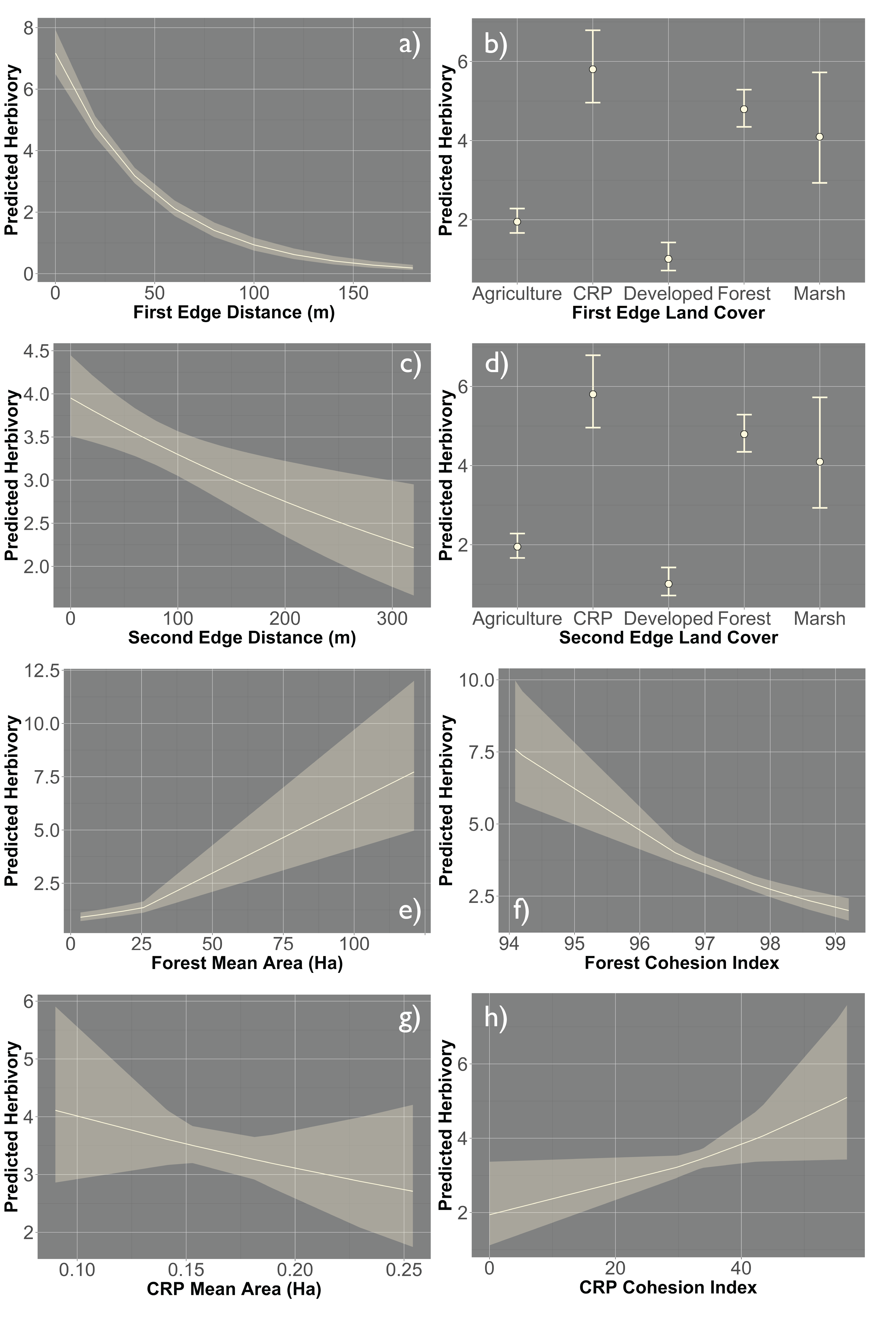
We mapped the proportion of herbivory and average plant height utilizing the GPS data collected. Utilizing ArcGIS, we used Empirical Bayesian Kriging to map a smooth surface of proportion of crop damage and average plant heights across the entire field. Statistically, we constructed a hierarchical explanatory model using a generalized linear mixed effects model that incorporates patch-level, class-level, and landscape-level metrics to explain spatial variability in crop damage present both within the field and between fields. Patch-level metrics included in the model are distances to both the nearest and second nearest edge as well as the landcover class of these edges. Class-level and landscape-level metrics were calculated from landcover classifications of buffer zones around each field. We utilized the USDA's 2021 National Cropland Data Layer for landcover classification, landcover types utilized were corn, sorghum, soybean, CRP, forest, shrub, developed, wetland and open water. Utilizing ArcGIS we clipped this layer to a constructed 220 hectare buffer zone (average home-range of female white-tailed deer in this region (Eyler 2001)). Each farm's clipped landcover classification file was then be imported into R studio, utilizing the 'landscapemetrics' package both class-level and landscape-level metrics were calculated for each field (Figure 2). Class-level metrics calculated for each field include mean area, core area index, percent of the landscape, patch cohesion index, patch density, percent of like adjacencies, splitting index, perimeter to area ratio and contiguity index for each landcover class present in the landscape (CRP, forest, etc.). Landscape-level metrics calculated for each field included core area index, total edge, patch cohesion index, connectance, number of patches, percent of like adjacencies, relative mutual information, Shannon’s evenness index, fractal dimension index and contiguity index. These metrics were included to incorporate a wide range of different types of metrics (shape, diversity, complexity, aggregation, area, and shape) to highlight what characteristics of the surround landscape influence crop damage. We reduced the number of variables incorporated into our models based off the overall correlation amongst variables. This resulted in 5 landscape-level variables and 2 class-level variables being utilized in the construction of the model. Allowing us to better understand how factors within the field as well as factors in the landscape surrounding the field influence how crop damage occurs across the field.
Initial trial sampling efforts were conducted in late August to early September 2020 at 2 farm sites (Barneck Farm and Anderson Farm) a total of 17 fecal pellets were collected. In March 2021 to May 2021 with the help of extension agents in Somerset County, we were able to connect with 5 other farmers experiencing heavy crop damage due to deer that were willing to allow us to use their farms as sites in our study. Starting in Late May/ early June 2021 we began collecting fecal pellets across 7 farmers on the Lower Eastern Shore of Maryland. We conducted another sampling effort in late August/ early September prior to the start of hunting season. A total of 62 fecal pellet samples were collected in June and 61 fecal pellet samples in late August/ early September across all 7 farms. A final sampling effort was conducted in late February/ early March of 2022 prior to any vegetation being present on the agricultural fields and 62 fecal pellet samples were collected across all 7 farms sampled. At the end of 2022 we have collected a total of 185 fecal pellet samples. All 185 samples have been processed and DNA extractions have occurred. However, upon sending samples off to the George Washington Genomics Core to be amplified and sequenced, quality control checks highlighted issues with the overall quality of the DNA in the samples. The overall plant DNA was highly degraded, as a result amplicon lengths of the target genes were too short to successfully amplify the plant DNA. Due to the inability to amplify the plant DNA, sequencing the DNA was unsuccessful. This was an unforeseen outcome of this study and the overall degradation of the DNA present in the samples may be a result of the lag time between sample collection and storage. Although samples were stored in a transport and storage medium that preserves the samples, the duration between collecting the samples and storing them in -70°C freezer was lengthy due to the number of fields sampled. This extended period may have provided time for samples to degrade.
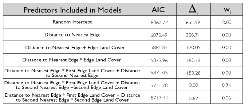
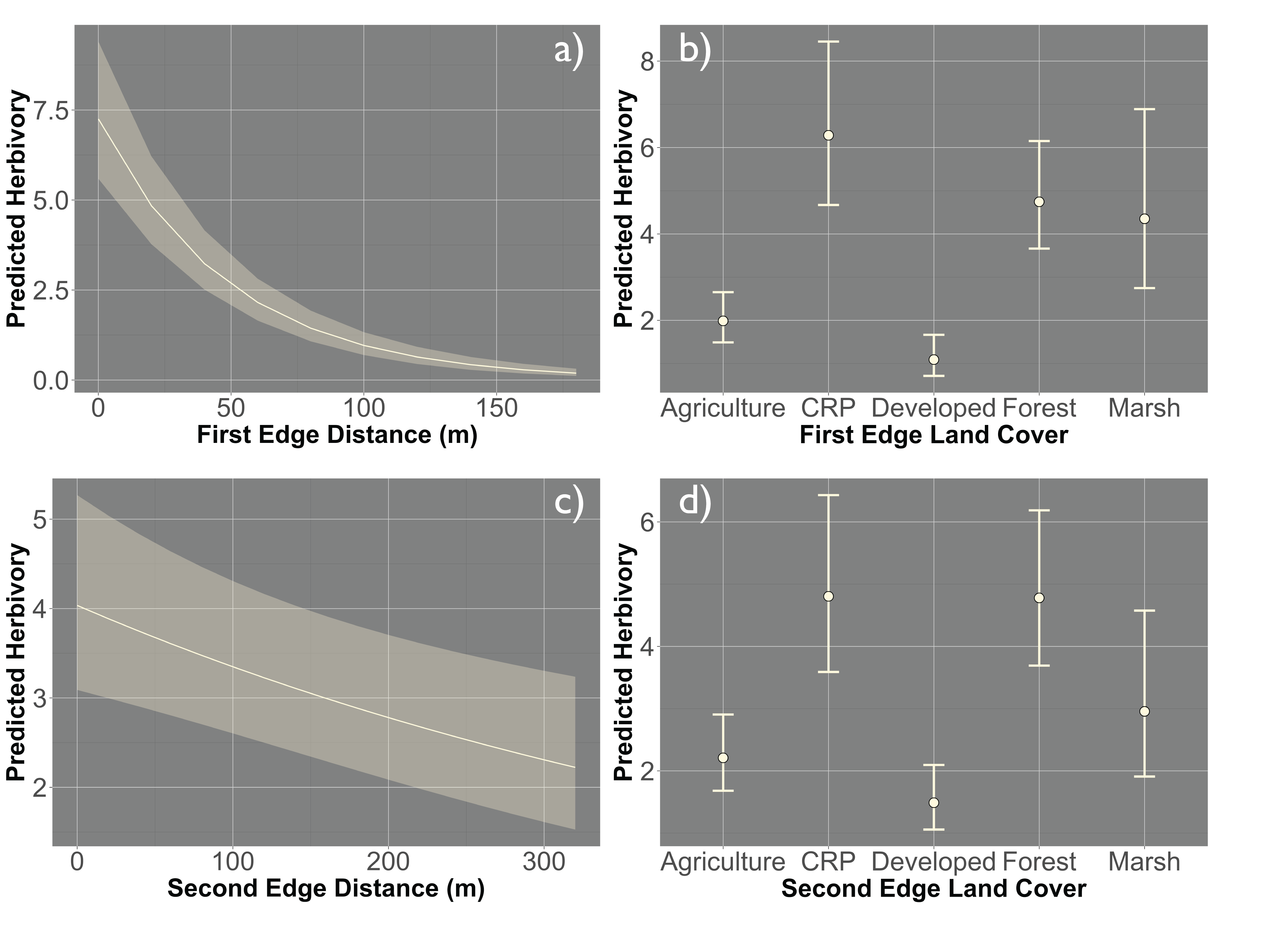
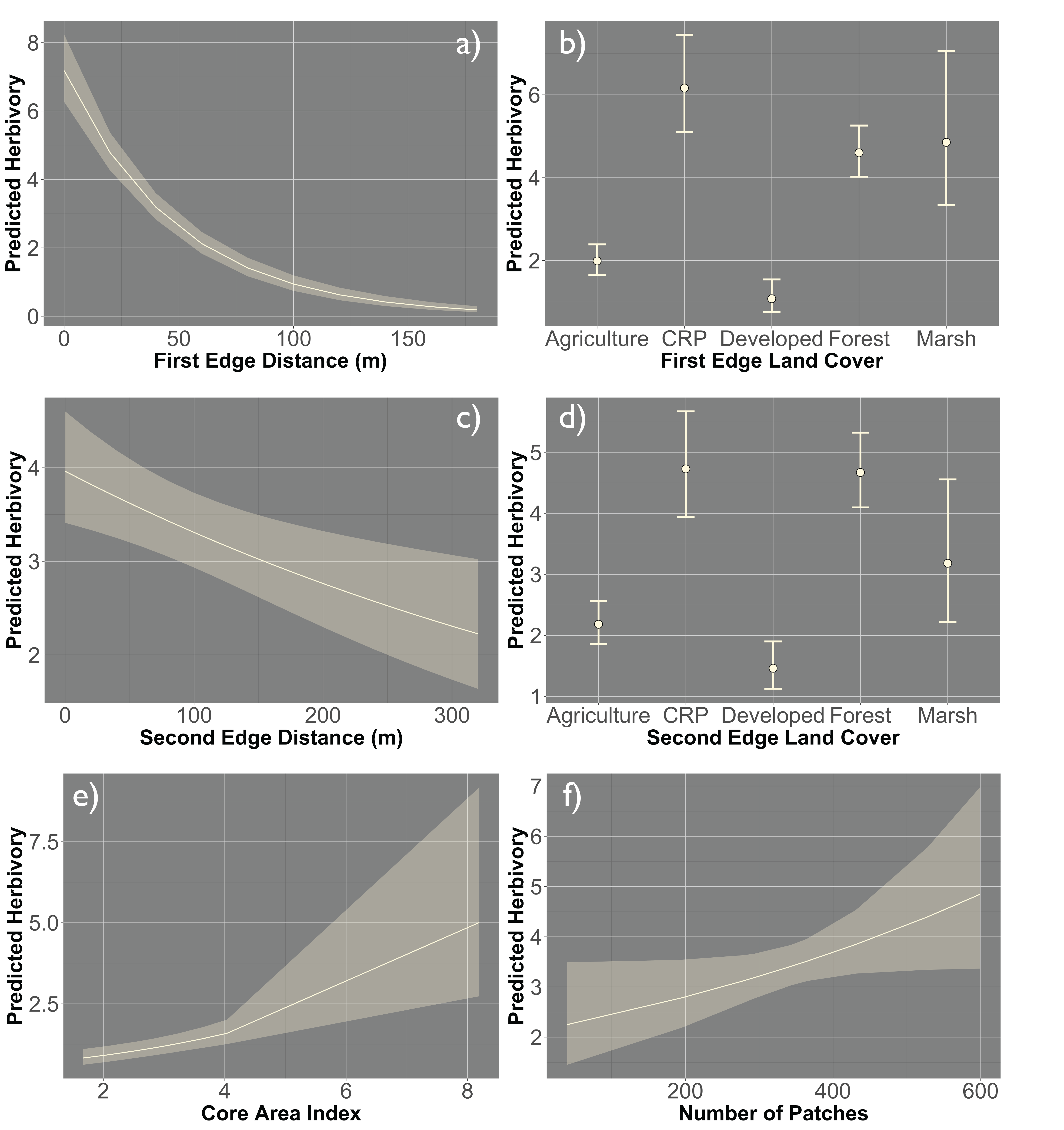
Due to the impasses relating to Objective 2, we decided to not only collect fecal pellets on the farm sites but also survey a select number of fields on each farm for crop damage in 2021. A total of 10 field were surveyed across the same 7 farms that we collect fecal pellets from. Across each field we sampled 120-180 randomly distributed points (depending upon the number of edges and corners the field had). We then utilized this data and Empirical Bayesian Kriging techniques is ArcGIS to be able to produce smoothed maps of crop damage and plant height of the entire field. We found that there is a high level of spatial variability present across the field, with certain regions experiencing higher levels of crop damage then others (Figure 1). In particular, the edges and corners experienced highest levels of herbivory (45-80% of plants experiencing herbivory). Crop damage was not limited to only the edges and corners but in some fields extended well into the interior (0-55% of plants experiencing herbivory) (Figure 2). To understand variability in crop damage within the field we constructed generalized linear mixed effects models that incorporated patch-level metrics which included distances to both the nearest and second nearest edges as well as the edge's landcover composition. We found that the best model based off Akaike Information Criterion (AIC) included the distance to both edges as well as the landcover composition (Figure 3). Significant terms in the model included distance to the nearest edge, nearest edge land-cover, distance to the second nearest edge and second nearest edge land-cover. The output of this model showed that herbivory decreased dramatically as distance to the first edge increased whereas it decreased more much less rapidly as distance to the second edge increased. It also showed the edge composition of the first edge impacted herbivory with forest, CRP and marsh edges had a more pronounced impact on herbivory than developed or agricultural edges (Figure 4).
However, there was a high level of spatial variability in crop damage between fields, highlighting the possibility that the surrounding landscape in which a field occurs could influence the level of crop damage on that field. To address how the surrounding landscape could influence crop damage we utilized a generalized linear mixed effect model framework to create hierarchical models that incorporated the patch-level model above (which we refer to as our field model) as well as landscape-level metrics for the entire field. We included core area index (landscape area metric), number of patches (landscape connectivity), contiguity index (landscape shape metric), relative mutual information (landscape complexity) and Shannon Evenness Index (diversity metric) in our model. We found the best model based off AIC included core area index and number of patches ( 0.22; Figure 5) although a model incorporating just contiguity index showed similar support ( 0.20; Figure 5). All terms that were significant in the field model remained significant after including the landscape metrics, as well as both the core area index and the number of patches were significant. The relationship between predicted herbivory and distance to the nearest edge, nearest edge land-cover, distance to the second nearest edge and second nearest edge land-cover remained consistent with the field model. The output of this model showed that as core area index and the number of patches increased in the landscape so did the predicted herbivory (Figure 6).
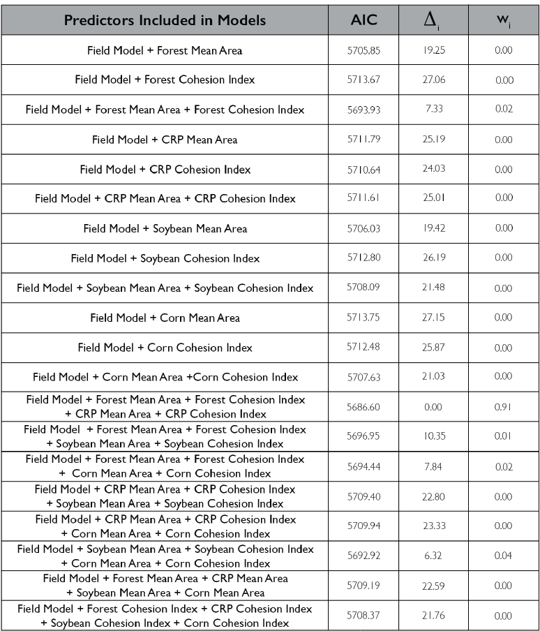
Lastly, we looked at how including class-level metrics impacts the herbivory experienced by the field, we again utilized a generalized linear mixed effect model framework to create a hierarchical model that incorporates the patch-level model as well as class-level metrics. We primarily examined the 4 most prevalent land classes in our landscape (Forest, CRP, Soybean and Corn). Models included various combinations of mean area and cohesion index (connectivity metric) of the four land-use types. The model incorporating forest mean area and cohesion index as well as CRP mean area and cohesion index showed the strongest support 0.91; Figure 7). Again, model terms that were significant in the field model remained significant after including the class metrics, forest mean area and cohesion index as well as CRP mean area and cohesion index were also significant in the class model. The relationship between predicted herbivory and distance to the nearest edge, nearest edge land-cover, distance to the second nearest edge and second nearest edge land-cover remained consistent with the field model. Predicted herbivory increased with greater forest mean area in the surrounding landscape and decreased with increased forest cohesion index (Figure 8). The opposite relationship was present for CRP, predicted herbivory decreased with greater CRP mean area and increased with greater CRP cohesion index (Figure 8).
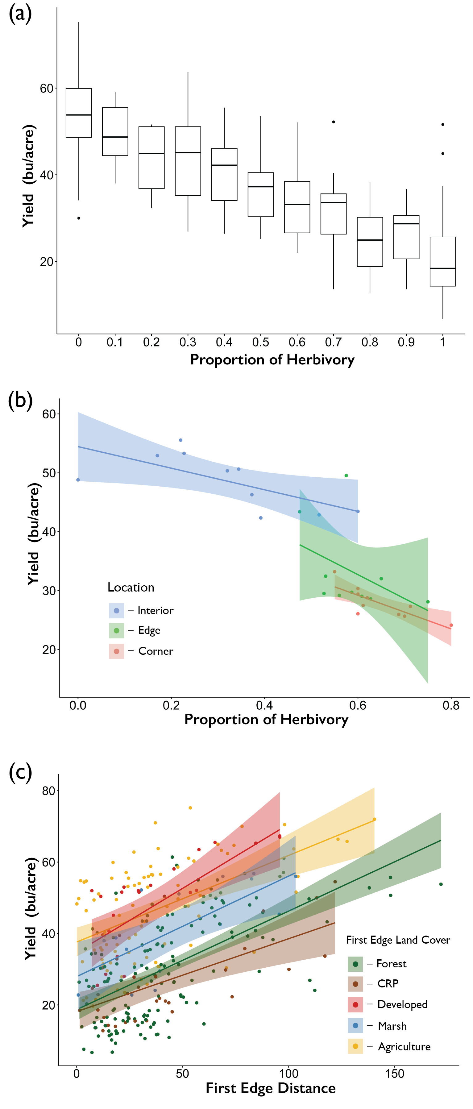
The yield of soybeans was influenced by damage experienced by white-tailed deer. We found that as the proportion of plants experiencing crop damage increased the overall yield decreased (Figure 9). The average yield when no plants experienced damage was 53.7 ± 9.3 (mean ± se) bushels per acre across our ten farms, whereas when all plants experienced damage, the average yield dropped to 20.1 ± 8.2 bushels per acre. The impacts of deer herbivory on yield were not constrained to just the edges and corners of the field, across all locations even the interior as the proportion of plants experiencing herbivory increased overall yield declined (Figure 9). Furthermore, edge land use influenced the distance into the field that the effects of deer damage had on yields. Yields increased as the distance to the nearest edge increased regardless of the edge land use, however forest and CRP edges had reduced yields relative to the other land use types (Figure 9).
Overall, we found that the most intense herbivory occurred in the corners and edges of agricultural fields. However, field interiors did not remain unscathed with 19% of soybeans experiencing depredation by white-tailed deer. In addressing hypotheses 1 and 2, we found that the land uses of the edges influenced the prevalence of damage experienced by the field. Edges that were CRP, forest, and marsh experienced higher levels of damage compared to agricultural and developed edges. As such field configuration did impact the level of crop damage occurring within the agricultural field, edges comprising other agriculture had reduced levels of damage compared to other land-use types. Configuring agricultural fields in a manner in which they border other agricultural fields could reduce the impacts of deer predation. In addressing hypothesis 3, we found that the configuration of the broader landscape did influence the proportion of crop damage the entire agricultural field experiences. Greater quantities of core area and number of patches in the landscape increased crop damage. The overall fragmentation of the landscape plays a significant role in influencing the intensity of damage experienced by the field. Lastly, in addressing hypotheses 4 and 5, the quantity and connectivity of forest and CRP in the surrounding landscape had a pronounced effect on crop damage. As the overall forest mean area increased and connectivity of those patches decreased crop damage increased, the opposite relationship was present for CRP, as the overall mean area decreased, and connectivity increased crop damage increased. Indicating that large fragmented forested patches and small interconnected CRP patches increase the intensity of damage. These results highlight the importance of considering the role the surrounding landscape plays not just the composition of the landscape but also the overall connectivity of landscape as well.

The overall aim of this study was not only to better understand the influence the surrounding landscape plays in driving white-tailed deer damage but to address many of the perceptions and concerns farmers have about how the surrounding landscape influences crop damage. All the participating farmers in this study had preconceived perceptions on how the surrounding landscape influences crop damage. We were able to distill our findings down to 6 questions frequently asked by the farmers in our system. Through directly addressing these perceptions, our goal is to provide actionable evidence to farmers about what does and does not influence the crop damage experienced by their agricultural fields.
Does crop damage only occur along the edges of agricultural fields?
We found that the most intense herbivory damage occurred in the edges and corners of the agricultural field. Although interiors of fields were impacted by crop damage with 19% of soybeans experiencing damage due to white-tailed deer. While most of the damage inflicted by deer will occur near the edges of fields due to the proximity of escape cover for deer, the interior of fields may experience damage especially if the overall size of the field is reduced.
Does having field edges of CRP and forest increase the crop damage in the agricultural field?
The land-use of the edges influenced the extent of damage in agricultural fields, with CRP, forest, and marsh edges experiencing higher levels of damage relative to agricultural and developed edges.
Do alterations to the landscape by neighboring landowners impact crop damage experienced by the field?
When looking at the influence of the broader landscape, rates of crop damage were best predicted by core area index of all land-use types and the number of patches in the landscape. More core area as well as a greater number of patches present in the landscape increased crop damage experienced by the field. A greater quantity of core area in the landscape means less edge habitat between different patch types. A greater number of patches indicates greater fragmentation of the landscape.
Does the presence of large tracts of forest in the region promote or inhibit crop damage?
When looking at the influence of specific land-uses on crop damage, forest area did play a significant role in influencing crop damage experienced by the field. However, it was not only forest area but also forest connectivity that impacted crop damage occurring in the field. As forest mean area increased and connectivity decreased in the landscape, the overall damage increased. Although a lot of attention is given to the influence forests have on crop damage, we found that CRP was another influential land-use affecting crop damage. We found that CRP has the opposite relationship, as CRP mean area decreases and connectivity increases overall damage increases.
Does crop damage significantly reduce the overall yield on their farms?
Crop damage inflicted by white-tailed deer impacted yield, as the proportion of plants experiencing herbivory increased the estimated yields declined. This relationship between browse damage and yield was present regardless of where the damage occurred in the fields (Interior, Edge, or Corner). Yields on edges and corners where browse pressure was the highest were reduced relative to the interior of fields. However, these effects may be exacerbated by environmental conditions present on field edges that impact yield synergistically. We also found a relationship between distance to the edge and yield, across all 5 edge land-uses yields increased as distance to the edge increased. Yet, forest and CRP edges had reduced yields relative to agricultural, developed and marsh edges.
What can the farmer do to mitigate the impact of white-tail deer on their farms?
It is vital that farmers know the influence the broader landscape plays in mitigating the effects of crop damage. Individualistic decision-making by the farmers can have a pronounced effect on the impact white-tailed deer have on their farms. We found that CRP, forest, and marsh edges had greater crop damage relative to other edge land-uses. Strategies that minimize edges comprising these land-uses could be utilized to reduce depredation. White-tailed deer preferentially browse on early successional habitat, farmers can reduce crop damage by increase the quantity of edge habitat and reducing large core areas present in the landscape. Thus, providing deer with alternative food sources in the landscape. Farmers can reduce crop damage by also inhibiting the further fragmentation of the landscape and isolation of deer surrounding their farms. Thus, allowing deer to move across the landscape and not be isolated to their farms. While we don’t advocate for removing forested habitat to reduce potential agricultural damage, increasing the connectivity of forested habitat in the surrounding landscape could also reduce the effects that large, forested regions have on depredation of crops. Lastly, where and how much CRP is present on their farms is a decision farmers can have that directly impacts crop damage. We found that increasing the amount of isolated CRP in the landscape could act an alternative food source for white-tailed deer reducing depredation on agricultural species. Farmers frequently convert edges of their field into CRP due to reduced productivity often because of increased depredation by deer. However, these decisions may only exacerbate the damage experienced by reducing the overall acreage of the field while simultaneously increasing the amount of CRP edge.
Education & outreach activities and participation summary
Participation summary:
This project leveraged the outreach program of a larger project funded by the USDA’s National Institute for Food and Agriculture (NIFA) that is researching the impacts of saltwater intrusion on agricultural fields in the Lower Eastern Shore of Maryland. The NIFA project has annual stakeholder meetings each spring in which farmers, extension agents, and other agricultural professionals participate, and I have had the opportunity to share my research results with this group. Unfortunately, due to COVID guidelines, this stakeholders meeting did not occur in 2021. However, in 2022 this meeting was held virtually with farmers, agricultural extension agents, and other researchers. I presented preliminary results during this meeting and talked with farmers about the issues they face regarding crop damage. In February 2023, I presented completed results from my crop damage surveys in person to stakeholders.
In 2022, I also participated in an informal gathering of local farmers that one of the farmers that I collaborate with held. In which we discussed the issues of crop damage, what my research is trying to address, and issues they are facing regarding the problem of crop damage. I also presented results from my crop damage field surveys to the 29th Annual Wildlife Society Conference in Spokane, Washington. At which I talked with researchers and land managers from both federal and state wildlife and agricultural agencies about the impacts of crop damage as well as utilizing the methodology I developed to survey crop damage more accurately.
In December 2023 and January 2024, I visited all the farmers that participated in the study to highlight the results we found in our study. This included farm visits in which both the participating farmers and neighboring farmers attended. We not only discussed the results of the study but also how the decisions made by the farmer can directly influence the impact crop damage has on their fields. I highlighted ways farmers can mitigate these impacts beyond trying to reduce deer populations on their farms through crop damage permits.
Project Outcomes
Crop damage is a persistent issue faced by farmers nationwide that impacts agricultural sustainability by affecting the economic viability of their farms and frequently putting them at odds with regional conservation efforts. Crop damage can often result in staggering losses to farmers in the form of crop damage with little recourse to mitigate these effects. Farmers often view their only solution to mitigate browsing losses is through crop damage permits and attempting to reduce the local deer population. However, deer populations occur over larger scales than a single property, as a result attempting to reduce the population frequently fails in mitigating the damage occurring to their farms. Thus, conflicts between farmers, deer, and local and regional wildlife managers often arise. These conflicts often put farmers at odds with regional and statewide conservation efforts, particularly when it comes to the management of white-tailed deer. Through providing adaptive management options to farmers, our research attempts to lessen the financial burden that comes with crop damage through providing farmers with alternative options to mitigate the effects of crop damage. Through alterations to their farms like minimizing certain edge types (forest, CRP, marsh), limiting landscape fragmentation, and being strategic when it comes to enroll certain parcels into CRP, farmers have methods beyond local population control to minimizing the effects of white-tailed deer. These options allow for farmers to reduce the financial impact crop damage inflicts as well as possibly reduce the conflict between regional conservation efforts and local farmers. Thus, promoting sustainable agricultural for the farmers in the form of economic viability of their farms.
Three of the farmers that were a part of the study and two farmers that were participants of outreach events acknowledged a change in attitude and knowledge about the issue of crop damage inflicted by white-tailed deer. All five of these farmers presumed that reducing deer densities through crop damage permits was the only option to mitigate the intense losses they experienced on their farm. Although they all acknowledged that their efforts to reduce deer densities through crop damage permits did not seem to be either sustainable (due to the financial burden of constantly monitoring their fields for the presence of deer and amount of time spent on this task) or effective (as deer from the surrounding landscape would often fill the void left by removing the deer). After conversations with these farmers and showing them the results of this study, they all acknowledged the importance of the surrounding landscape in influencing the prevalence of crop damage inflicted on their farm. They acknowledged that decisions they make in the landscape, such as where they place CRP easements or the prevalence of forested edge along their fields can have a significant impact on the damage those fields experience. Two of the farmers that were a part of the study and one farmer that was a participant of outreach took it a step farther and decided to adapt new practices when it comes to mitigating crop damage inflicted by white-tailed deer. These farmers are no longer converting portions of their field that are no longer productive due to intensive crop damage into CRP, thus mitigating the amount of CRP that surrounds their active farm fields. They now understand that these decisions result in smaller fields which allows for the extent of deer damage to extend farther into their fields and impact field interiors that would normally not experience crop damage. As well as provide bedding habitat for white-tailed deer in close proximity to their agricultural fields. However, all five farmers have acknowledged that factors beyond local deer density can have a profound impact on crop damage and provide them with more options to mitigate these damages.
Throughout this project, my attitude and awareness about sustainable agriculture was transformed. Through the many conversations with participating farmers, I have realized the plethora of challenges farmers in our system face in making their farms viable. Farmers must factor in unforeseen consequences in their decision-making and accept that these decisions can have a profound impact on the financial viability of their farms. Often farmers are positioned at crossroads when it comes to making decisions that could impact their farm, and often there is limited information available to help inform farmers about how these choices can impact them. The need to conduct research to address pertinent questions farmers have on sustainable agriculture is urgent. Most importantly, the research on sustainable agriculture needs to be tailored to the farmer’s needs, which this project is a prime example of. This project came to be because of work done by my advisor on another complex issue farmers on the Delmarva peninsula, the impacts of saltwater intrusion on farming. However, through conversations with farmers about other issues they were facing on their farms, it was realized that understanding the influence herbivores play in these systems was an important knowledge gap that the farmers needed addressed. Overall, through this project I realized sustainable agriculture is difficult for many farmers and research on topics farmers need answers to is a vital first step in helping them overcome these challenges.
My future direction for research and career is primarily focused on understanding the effects sea-level rise and saltwater intrusion have on coastal plant communities. This includes the impacts sea-level rise has on coastal agriculture but also many other ecosystems in the region being impacted by climate change. However, this project has allowed me to understand the challenges farmers in these systems face and the need to help them address many of the issues that are currently arising now and may arise in the future due to the impacts of climate change.