Final report for GW19-190
Project Information
The loss of nitrogen (N) from crop fields is a national issue that plagues not only terrestrial and aquatic ecosystems, but human and animal health as well. The over application of fertilizer on farms across the country results in N that is left unused by crops, acidifying soils and flowing into waterways in addition to loss of revenue for the producer. Using variable rate N application (VRA) to site-specifically apply fertilizer, rather than application of a uniform rate, has potential to reduce the amount of N applied to fields and increase grower profits. This study sought to determine the amount of nitrogen fertilizer to place at each point in the field to maximize profit and at the same time minimize nitrogen lost to leaching through the soil profile. Full-field variable N rate experimentation conducted with precision agriculture technologies (VRA, yield monitors and protein sensors) numerous GIS, climate, and remote-sensing based covariates andspatiotemporally dense soil and plant sampling and N analysis were used to construct equations to predict optimum N rates in dryland small grain agroecosystems. The predictive equations were used in a software developed for this project to create site-specifically optimized nitrogen fertilizer application rates based on maximized net-return and minimized nitrate pollution under different climatic and weather scenarios. Site-specific N fertilizer management were compared with other application approaches based on net returns to producers and pollution potential tradeoffs. In all fields, adoption of site-specific N fertilizer management increased farmer profits compared to a uniform farmer selected N fertilizer rates. Using site-specific N management also tended to reduce the amount of total N applied across most fields. Annual workshops and reports for producers and the public happened every year to disseminate research results and a software package that automates the data management, analysis, and generation of optimized prescriptions has been developed. Future work will involve migrating the software package from the R environment into a web-based application that is user-friendly and accessible for farmers and crop consultants.
The primary research goal was to estimate nitrogen use efficiency (NUE) from each point in a wheat field where yield is reported by the combine yield monitor and grain protein analyzer. This required measurement of NUE in representative dryland wheat systems of Montana and extrapolating the losses using a predictive model. To achieve this goal, the specific objectives were:
- Quantify the relationship of crop (dryland winter wheat) yield and grain protein with N fertilizer rates from variable rate application (VRA) on-farm experiments (OFE) utilizing grain yield combine-harvester monitor data and protein analysis along with GIS, climate, and remote sensing-based covariates.
- Determine NUE after soil and plant inventories by calculating a N mass balance using intensive soil and plant tissue sampling.
- Predict NUE at each yield/protein monitored point using geostatistical techniques.
- Quantify and package site-specific optimized N fertilizer application rates based on maximized net return and minimized pollution potential via leaching, surface runoff and atmospheric loss into a field-specific software application available for use by growers.

Cooperators
- - Producer
- - Producer
Research
Study Site
Seven fields in Montana representing different climatic and soil regions were selected from a larger population of fields for which data is being collected for the OFPE project led by Dr. Bruce Maxwell (Fig. 1). The benefit of using producers who have prior experience and participation in site-specific management with OFPE is their experience in research management on their fields as well as our access to their historical data. Fields were selected based on the crop grown in 2020 and 2021 (winter wheat) and on the quality and promptness of data collection by the producers. Additionally, producers covered a three different cooperator farms, generating a dataset with measurements in different geographic locations.
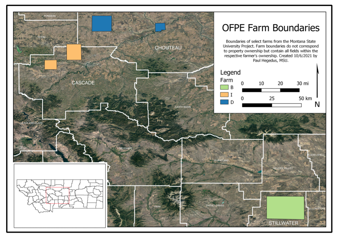
Fig. 1. Map of OFPE farm boundaries of collaborators with Montana State University. Colors represent different farmers, while shapes represent areas in which their respective fields fall within. The letter identifiers match those in Table 1.
All fields were under OFPE experimental management in either 2016, 2018, and 2020 or 2017, 2019, and 2021 (Table 1). Fields selected were required to have experimental N data available from at least three years. Nitrogen fertilizer rates were experientially applied in the field in blocks varying from 400 – 600 feet long and as wide as the farmer’s fertilize sprayer or spreader width, varying from 60 – 120 feet wide. Rates were randomly placed throughout the field, stratified on previous yield, protein, and N applied.
Table 1. Collaborator farm ID (Fig. 1), field names, field size (acres), crop harvest history, years of N experimentation. The letter identifier for the Farm corresponds to Figure 1.
|
Farm |
Field |
Field size (ha) |
Crop History1: 2014 / 2015 / 2016 / 2017 / 2018 / 2019 / 2020 / 2021 |
Years N rate treatment |
|
B |
B1 |
79 |
SF / WW / CF / WW / CF / WW / CF / WW |
2017, 2019, 2021 |
|
B2 |
94 |
WW / CF / WW / CF / SF / WW / CF / WW |
2016, 2019, 2021 |
|
|
B3 |
64 |
SW / CF / WW / CF / WW / CF / WW / CF |
2016, 2018, 2020 |
|
|
D |
D1 |
46 |
CF / WW / CF / WW / CF / WW / CF / WW |
2017, 2019, 2021 |
|
|
D2 |
48 |
WW / SW / WW / CF / WW / CF / WW / CF |
2016, 2018, 2020 |
|
|
D3 |
20 |
SW / SW / WW / CF / WW / CF / WW / CF |
2016, 2018, 2020 |
|
I |
I1 |
94 |
SW / CF / WW / CF / WW / CF / WW / CF |
2016, 2018, 2020 |
|
1 WW = winter wheat, CF = chemical fallow, SW = spring wheat, SF = safflower |
||||
The response variables of interest were crop productivity (yield in bushels per acre) and quality (grain protein percent), both of which were gathered from monitors mounted in the cab of the farmer’s combine harvesters. Yield was collected about every three seconds while protein was measured about every ten seconds. Yield is related to price received for wheat based on volume (bu), however protein in winter wheat is judged based on a nonlinear scale. On typical years, protein content above 11.5% is rewarded with a 2 cent per half point protein increase on the base price received, however if protein is below 11.5%, the price received is decreased by 8 cents per half point protein down to 9.5%. Thus, the combination of quantity and quality of the winter wheat crop influences farmer net returns. Farm equipment used in this study varied between farmers, with one using John Deere and the other using Case. All yield monitors are calibrated every spring by the farmers, according to their respective manufacturing instructions. Grain protein content was measured with Next Instrument’s CropScan 3300H near infrared monitor (product citation) which was installed, maintained, and calibrated by Triangle Ag Crop Consultants (website citation). Both yield and protein data are subjected to proprietary cleaning practices according to the software of the machine used to make the measurement. In addition to the yield, protein, and as-applied N data that were collected from the machines on the field, remotely sensed covariate data from open sources was gathered (Table 2). These data were gathered or derived from Google Earth Engine (Gorelick et al. 2017) and aggregated together at the locations of the observations in the yield and protein datasets.
Table 2. Table of covariate data types gathered from Google Earth Engine to enrich the crop yield and protein datasets gathered from on-farms.
|
Data Type |
Data Sources |
Resolution |
Years Collected |
Description |
|
Normalized Difference Vegetation Index (NDVI) |
Landsat 5/7/8 |
30m |
L5: 1999-2011 L7: 2012-2013 L8: 2014 - present |
Landsat is an ongoing USGS and NASA collaboration. Bands (NIR, red) L5/L7: B4 and B3 L8: B5 and B4 |
|
Normalized Difference Water Index (NDWI) |
Landsat 5/7/8 |
30m |
L5: 1999-2011 L7: 2012-2013 L8: 2014 - present |
Landsat is an ongoing USGS and NASA collaboration. Bands (NIR, red) L5/L7: B2 and B4 L8: B2 and B5
|
|
Elevation |
USGS NED |
~10m (1/3 arc second), ~23m (3/4 arc second) |
1999-present |
USGS National Elevation Dataset. Measured in meters. |
|
Aspect |
USGS NED |
~10m (1/3 arc second), 30m |
1999-present |
Direction the surface faces, function of neighboring elevations, in radians. Also calculated for each E/W and N/S direction as cosine and sine. |
|
Slope |
USGS NED |
~10m (1/3 arc second), 30m |
1999-present |
Rate of change of height from neighboring cells, in degrees. Measured in degrees. |
|
Topographic Position Index (TPI) |
USGS NED |
~10m (1/3 arc second), 30m |
1999-present |
Measure of divots and low spots as a function of neighboring elevation. |
|
Precipitation |
DaymetV3 |
1km |
1999-present |
Estimates from the NASA Oak Ridge National Laboratory (ORNL). Measured in mm. |
|
Growing Degree Days (GDD) |
DaymetV3 |
1km |
1999-present |
Estimates from the NASA Oak Ridge National Laboratory (ORNL). |
|
OpenLandMap |
bulkdensity |
250m |
1999-present |
Soil bulk density (fine earth) 10 x kg / m3 averaged over 6 standard depths (0, 0.1, 0.3, 0.6, 1 and 2 m). |
|
OpenLandMap |
claycontent |
250m |
1999-present |
Clay content in % (kg / kg) averaged over 6 standard depths (0, 0.1, 0.3, 0.6, 1 and 2 m). |
|
OpenLandMap |
sandcontent |
250m |
1999-present |
Sand content in % (kg / kg) averaged over 6 standard depths (0, 0.1, 0.3, 0.6, 1 and 2 m). |
|
OpenLandMap |
pH (phw) |
250m |
1999-present |
Soil pH in H2O averaged over 6 standard depths (0, 0.1, 0.3, 0.6, 1 and 2 m). |
|
OpenLandMap |
watercontent |
250m |
1999-present |
Soil water content (volumetric %) for 33kPa and 1500kPa suctions predicted and averaged over 6 standard depths (0, 0.1, 0.3, 0.6, 1 and 2 m). |
|
OpenLandMap |
carboncontent |
250m |
1999-present |
Soil organic carbon content in x 5 g / kg averaged over 6 standard depths (0, 0.1, 0.3, 0.6, 1 and 2 m). |
Crop Response Modeling
The first objective was achieved by characterizing the response and variation in yield and protein data to N fertilizer application using multiple statistical methods such as regression, Bayesian, and machine learning approaches. These models were fit using the large amounts of data collected from yield harvesters and protein analyzers mounted on the combine, and from aggregated 10m scale covariate data aggregated from the earth observation satellites.
Crop response models they use must be accurate for forecasting future crop responses and allow for quantification of the uncertainty in the forecast. To mimic reality, in which models need to forecast crop responses in a future year not represented in training data, a k-fold cross validation type design was used. Harvest, as applied fertilizer, and covariate data for each of the three years that every field underwent N fertilizer experimentation were collected as described above. The crop-fallow system practiced in all the fields means harvest data from experimental years are available every other year on a 2016, 2018, 2020 or 2017, 2019, 2021 schedule. For each field, three split cases with different data configurations were created where two years of data were used for training while data from one year were held out as a test set to evaluate the ability of the model to forecast crop responses in a year with observations unseen by the model (Fig. 2).
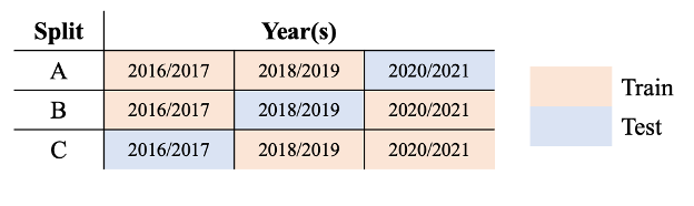
Figure. 2. Design matrix for data configurations applied to each field for all 5 model types. Orange cells represent the years used for training in each case and blue cells represent the year used for testing in each case.
Five parametric to non-parametric models that range from using frequentist, Bayesian, and machine learning approaches were fit to crop responses on each field. The models used were a modified version of a non-linear sigmoid model, generalized additive model (GAM), linear and non-linear Bayesian models, and a random forest regression model. For each field, each model type was fit individually using grain yield (kg ha-1) or grain protein concentration (%) as response variables with variable as-applied N fertilizer rates (kg ha-1) and covariates as predictor variables (Table 3). All analysis was performed in R (R Core Team, 2021), where the OFPE package was used for all data management and analysis (Hegedus, 2020). All covariate data in training datasets were tested to avoid aliasing and covariance between predictors.
Table 3. Identifiers for covariates in the models below, the covariate’s data type and a description of the covariate.
|
Covariate ID |
Data Type |
Description |
|
aspectcos |
Aspect |
Aspect in the E/W direction |
|
aspectsin |
Aspect |
Aspect in the N/S direction |
|
slope |
Slope |
Slope in degrees |
|
elev |
Elevation |
Elevation in meters |
|
tpi |
TPI |
Topographic Position Index |
|
precpy |
Precipitation |
Precipitation summed from the water year two years prior to observed data (mm) |
|
gddpy |
GDD |
Growing degree days summed from the year prior |
|
ndvipy |
NDVI |
Maximum Normalized Difference Vegetation Index from across the prior year |
|
ndvi2py |
NDVI |
Maximum Normalized Difference Vegetation Index from across two years prior |
|
ndwipy |
NDWI |
Maximum Normalized Difference Water Index from across the prior year |
|
ndwi2py |
NDWI |
Maximum Normalized Difference Water Index from across two years prior |
|
bulkdensity |
Bulk Density |
Soil bulk density (fine earth) 10 x kg / m3 averaged over 6 standard depths (0, 0.1, 0.3, 0.6, 1 and 2 m). |
|
claycontent |
Clay Content |
Clay content in % (kg / kg) averaged over 6 standard depths (0, 0.1, 0.3, 0.6, 1 and 2 m). |
|
phw |
pH of Water |
Soil pH in H2O averaged over 6 standard depths (0, 0.1, 0.3, 0.6, 1 and 2 m). |
|
watercontent |
Water Content |
Soil water content (volumetric %) for 33kPa and 1500kPa suctions predicted and averaged over 6 standard depths (0, 0.1, 0.3, 0.6, 1 and 2 m). |
|
carboncontent |
Carbon Content |
Soil organic carbon content in x 5 g / kg averaged over 6 standard depths (0, 0.1, 0.3, 0.6, 1 and 2 m). |
1) Modified Non-Linear Sigmoid Model (Beta Function)
The first model type was parametric and modified from a non-linear sigmoidal model called the beta function (Yin, Goudriaan, Lantinga, Vos, & Spiertz, 2003). Following the literature, a model that assumes an asymptotic nature of crop response curves to additional N fertilizer was tested here (Anselin, Bongiovanni, & Lowenberg-DeBoer, 2004; Reynolds, Drury, Phillips, Yang, & Agomoh, 2021; Yin et al., 2003). Initial tests compared the beta function to multiple forms of non-linear models including: hyperbolic, Richards, Gompertz, Weibull, and logistic forms. Selection of the beta function (Yin et al., 2003) over these other non-linear models was based on three factors; 1) the beta function yielded the lowest mean RMSE across fields for both yield and protein (Table 4), 2) the beta function required the least locking of parameters to facilitate convergence, and 3) the beta function captured the asymptotic response and a downturn of responses at high experimental N fertilizer rates.
Table 4. Results of the mean RMSE across the seven fields of yield and protein from each of the non-linear models tested with a randomly split training dataset with 70% of observations across three years for model fitting and a hold-out dataset with the other 30% of observations for predicting responses with new data and calculating RMSE.
|
Model |
Mean RMSE for Yield (kg ha-1) |
Mean RMSE for Protein (%) |
|
Beta Function |
1193.133 |
1.6214 |
|
Gompertz |
1219.139 |
1.6741 |
|
Hyperbolic |
1216.698 |
1.6771 |
|
Logistic 1 |
1205.729 |
1.6317 |
|
Logistic 2 |
1194.276 |
1.6236 |
|
Richards |
1205.265 |
1.6256 |
|
Weibull 1 |
1199.535 |
1.6389 |
|
Weibull 2 |
1252.273 |
1.7610 |
The beta model was modified by incorporating an intercept term to represent the response of the crop at zero N-rate. Additionally, a Gaussian spatial correlation structure on the UTM coordinates of observations to account for the spatial dependence of responses was included (De Bastiani, Mariz de Aquino Cysneiros, Uribe-Opazo, & Galea, 2015; Diggle & Tawn, 1998; Mardia & Marshall, 1984; Xia, Ding, & Wang, 2008). The beta function was fit using generalized non-linear least squares regression through the nlme package in R (Pinheiro, Bates, DebRoy, Sarkar, & R Core Team, 2021). Bottom-up feature selection was performed where predictors that did not contribute to a decrease in AIC by two units were omitted from the model. As crop responses differed across fields, not all beta functions fit for yield or protein for a given field and set of training years have the same predictors. All final models for each field were selected from the following beta function used for yield (kg ha-1) or grain protein concentration (%) forecasting, with a Gaussian process spatial correlation structure, and the predictors that influence the intercept term (α);
![]()
(1)
Where R is yield (kg ha-1) or grain protein concentration (%), α is the fit minimum yield at a zero N-rate, β is the fit maximum yield (asymptote) at high N-rates, N is the as-applied N-rate in kg ha-1, δ2 is the fit N-rate where β is approached, δ1 is the fit N-rate at the inflection point (center of the upturn of the curve), Gaussian(x, y) is the Gaussian process spatial correlation structure, and ε is random error assumed to be normal and independent N(0, σ2). The intercept term, α, was assumed to be influenced by all topographic variables and information from prior years;
![]()
(2)
Where α0 - α15 were coefficients for the intercept and covariate data listed in Table 3.
2) Generalized Additive Model (GAM)
Staying in the non-linear realm but relaxing assumptions on the shape of the model for crop responses, a generalized additive models (GAMs) was tested. Generalized additive models are a blend of semi-parametric generalized linear models with additive smoothing terms for modeling non-linear relationships between covariates and the response (Hastie & Tibshirani, 1986; Wood, 2017; Pinilla & Negrín, 2021). Despite their flexibility, the use of GAMs for modeling crop responses has been limited (Chen, O’Leary, & Evans, 2019; Estes et al., 2013; Joshi, Kazula, Coulter, Naeve, & Garcia y Garcia, 2021; Liew & Forkman, 2015). The GAMs for grain yield and grain protein concentration used gamma family distributions and thin plate splines with shrinkage for the basis functions on most of the covariates in Table 3. A gamma family distribution was selected to ensure that estimates and predictions were above zero in accordance with the reality of grain yield and grain protein concentration measurements. Shrinkage allowed estimated degrees of freedom to fall to zero, combining the model fitting and feature selection process. The only covariates that did not use a thin plate basis function were the spatial UTM coordinates, which were included as smoothing terms with a Gaussian process basis function to account for spatial autocorrelation (Gotway & Stroup, 1997; Guisan, Edwards, & Hastie, 2002; Holland, De Oliveira, Cox, & Smith, 2000; Zuur & Camphuysen, Kees, 2012). To account for non-constant variance found in initial model fits, a log link function was used. Models were fit using the mgcv package in R (Wood, 2003; Wood, Pya, & Säfken, 2016). As crop responses differed across fields, not all GAMs for yield or protein for a given field and set of training years have the same predictors but selected from the following initial GAM with a gamma family distribution and log link function;
![]()
(3)
Where R is the expected yield (kg ha-1) or grain protein concentration (%) with a gamma log link function, I is the intercept, f1 is the tensor product of the x and y coordinate (x, y) with a Gaussian process basis function, f2 is the tensor product of centered aspect in the E/W direction (aspectcos) and aspect in the N/S direction (aspectsin) with a thin plate shrinkage spline basis function, f3 – f17 are smoothing functions fit with maximum likelihood and thin plate shrinkage splines as the basis function for covariates listed in Table 3, and ε is the random error, assumed to be normal and independent N(0, σ2).
3) Non-Linear Bayesian Regression Model (Bayes NLR)
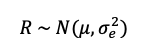
Two Bayesian models were also tested. Bayesian approaches are commonly applied for modeling crop responses (Besag & Higdon, 1999; Huang, Huang, Yu, Ni, & Yu, 2017; Jiang, He, Kitchen, & Sudduth, 2009; Lawrence et al., 2015; Nandram, Berg, & Barboza, 2014; Ramsey, 2020; J. C. Wang et al., 2012) but are also used for models that influence policy such as yield gap and potential (Prost, Makowski, & Jeuffroy, 2008) and commodity prices (Drachal, 2019). The first Bayesian model used was adapted from Lawrence, Rew, & Maxwell (2015). Two modifications were made to fit this dataset and scenario, including replacing electrical conductivity data with clay content, based on the correlation between the two properties (McBratney, Minasny, & Whelan, 2005). Second, the precipitation term used as a predictor for crop responses was constrained in this model to precipitation summed across the previous year, as only this data would be available when forecasting is required to make management decisions in an upcoming year. Finally, because this data represented scattered points across a field rather than a lattice grid structure in Lawrence et al., simultaneous spatial auto regression (SAR) was used rather than conditional auto regression (Ver Hoef, Hanks, & Hooten, 2017; Wall, 2004). The base of this model was identical to Lawrence et al. (2015) where grain yield and protein were assumed to follow a normal distribution;
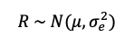
(4)
Where R was the grain yield (kg ha-1) or grain protein concentration (%) that followed a normal distribution with a variance, σε2, that followed an inverse gamma distribution;
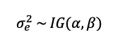
(5)
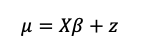
And the mean crop response, μ, was defined by a non-linear crop model;
![]()
(6)
Where N was the as-applied N-rate (kg ha-1), precpy and claycontent are defined in Table 3, and z was the SAR spatial random effect;
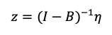
(7)
Where η had a mean E(η) ≡ 0 and Cov(η) ≡ σz2I. I was the identity matrix, and B was the n x n spatial dependence matrix between ni and nj where i ≠ j and i, j = 1, ..., n (Hooten, Ver Hoef, & Hanks, 2019).
All priors used were the same as in Lawrence et al., where the prior for σε2 followed a gamma distribution with 0.01 used for both shape parameters in (5). For β terms in (6), truncated normal distributions, TN(0, 1000), were used for all terms except where βmax = N(0, 1000). All Bayesian methods were executed in R using the Stan based brms package (Bürkner, 2021; 2018; 2017).
4) Bayesian Multiple Linear Regression Model (Bayes MLR)
The second type of Bayesian approach tested was a multiple linear regression (MLR) model. Based on initial exploration of the data (Hegedus & Maxwell, 2022), a normal distribution as the base of a SAR MLR model was used (Anselin et al., 2004; Hooten et al., 2019; Kissling & Carl, 2008; Ver Hoef, Petersen, Hooten, Hanks, & Fortin, 2018);
(8)
Where R was the grain yield (kg ha-1) or grain protein concentration (%), σε2 was identical in formation and priors as (5), and;
(9)
where β was the coefficient vector (β0, ..., βp-1) with p the number of predictors from Table 3, X is the n x p covariate matrix of covariate vectors, and z was the SAR random effect. To avoid overfitting, top-down feature selection was applied and omitted covariates where dropping them from the model reduced the AIC by more than two units. Thus, Bayesian MLR models vary in their covariates between fields and splits but are all fit from the same initial model;
![]()
(10)
Where predictor variables are covariates from Table 3 with uniform priors on coefficients β0 - β16 (Gelman, 2006), and the SAR spatial random error, z, defined in (7). As with the non-linear modeling, the Stan based brms package in R was used for Bayesian analyses (Bürkner, 2021; 2018; 2017).
5) Random Forest Regression (RF)
Random forest (RF) regression is an increasingly popular non-parametric machine learning method that has been used to model spatial data (Georganos et al., 2021; Jing, Yang, Yue, & Zhao, 2016; Li, Heap, Potter, & Daniell, 2011; Shi et al., 2015), specifically crop response data (Everingham, Sexton, Skocaj, & Inman-Bamber, 2016; Jeong et al., 2016; Lawes, Oliver, & Huth, 2019; Mariano & Mónica, 2021; Marques Ramos et al., 2020; Paccioretti et al., 2021; L. Wang, Zhou, Zhu, Dong, & Guo, 2016), where crop responses are estimated by the ensemble of regression trees using binary splits of observations based on covariate data. The ranger package in R was used for fitting and generating predictions (Wright & Ziegler, 2017). The predictors included in the RF models for yield and protein are in Table 3. To avoid over-fitting, top-down feature selection was performed where covariates were omitted if dropping them from the model resulted in an AIC decrease of over two units. The number of trees (ntrees) and the number of covariates sampled at each node (mtry) were optimized during the fitting process. To account for spatial effects, UTM coordinates were included as a variable definition following spatial random forest regression practices in the literature (Janatian et al., 2017; Langella, Basile, Bonfante, & Terribile, 2010; Walsh, Kreakie, Cantwell, & Nacci, 2017; Y. Wang et al., 2017).
NUE Sampling and Calculation
The second objective was approached using intensive soil and plant tissue sampling along with managerial control over the N fertilizer rates applied. Previous work and ongoing investigations led by Dr. Stephanie Ewing in the Judith River Watershed (JRW) of Montana has instigated reactive transport modeling undertaken with nitrate data collected with lysimeters in the JRW. This model, developed in R, assesses N loss pathways and their relationship with soil characteristics, weather, and management decisions. Insights from this model indicate that in a typical Montana dryland agroecosystem, soil water holding capacity has the greatest influence on soil regulation of N loss. This work informed the investigation of spatial relationships between data collected on-farms and from remote sensing will be investigated in OFPE fields to indicate portions of the field that exhibit characteristics of N loss. Under the assumption that soil water storage drives nitrate dynamics and N loss, spatial relationships between historic productivity and precipitation were evaluated in OFPE fields to estimate water holding capacity in subfield units. Four fields in Montana were subjected to intensive soil and plant biomass sampling to generate a dataset for spatially varying NUE across fields (Table 5).
Table 5. Collaborator farm ID (Fig. 1), field names, field size (hectares), crop harvest history, and the year sampled. The letter identifier for the Farm corresponds to Figure 1.
|
Farm |
Field |
Field size (ha) |
Crop History1: 2014 / 2015 / 2016 / 2017 / 2018 / 2019 / 2020 / 2021 |
Year Sampled |
|
|
B |
BSE |
79 |
SF / WW / CF / WW / CF / WW / CF / WW |
2021 |
|
|
B |
BS |
64 |
SW / CF / WW / CF / WW / CF / WW / CF |
2020 |
|
|
I |
MS |
46 |
CF / WW / CF / WW / CF / WW / CF / WW |
2021 |
|
|
D |
WH |
48 |
WW / SW / WW / CF / WW / CF / WW / CF |
2020 |
|
|
1 WW = winter wheat, CF = chemical fallow, P = peas, SW = spring wheat, SF = safflower, NA = Not Available |
|||||
The time and money required for detailed soil sampling are limitations on the ability of most farmers to assess N transport and soil characteristics within their fields. Based on the work of Sigler and John et al. in Montana small grain dryland agroecosystems, the thickness of fine textured soils, or simplified to soil water storage, is assumed to be a soil characteristic that influences variation of NUE within fields. If precipitation inputs exceed crop water uptake and soil water storage, nitrate leaching is hypothesized to be the dominant pathway of N loss because nitrate that has not been taken up by the crop or retained in the soil will be transported below the crop rooting depth in well-drained soil. If N limitation of dryland small grain agroecosystems is a function of leaching loss with excess N application, then soil water storage (WHC) will dictate yield capacity when N fertilizer application exceeds crop requirements. Thus, soils with high WHC will contribute to higher yields and less nitrate leaching of excess fertilizer because the water is retained in the root zone.
To account for the variation in NUE explained by soil water storage, a high spatial density estimate of WHC was created. If soil water storage is a function of the depth of fine textured soils, then consistency in productivity over time at a specific point in a field could reveal insight into WHC at that point. While no studies have found have linked historical NDVI imagery to NUE or WHC, Araya et al. used NDVI to estimate available water content, indicating the promise NDVI has for estimating soil properties (Araya, Lyle, Lewis, & Ostendorf, 2016). The implications for identifying areas of a field at risk of N loss from freely available remotely sensed data benefits farmers by providing information on where NUE is potentially low, which can inform site-specific N fertilizer management decisions.
The fields used in this study were classified into WHC zones that were used to stratify soil and plant biomass sampling. Normalized Difference Vegetation Index (NDVI) was derived from satellite imagery from 2000 – 2021. Landsat imagery was collected on 30m x 30m raster grids, a coarser resolution than satellites such as Sentinel-2 however, was chosen for the length of imagery history available (Table 6). Landsat 7 data was only used for one year due to a failure in the Scan Line Corrector causing a gap-filled zig-zag pattern during data collection.
|
Program |
Resolution |
Years Available |
Years Collected |
|
Landsat 5 |
30m |
March 1984 – May 2012 |
1999 – 2012 |
|
Landsat 7 |
30m |
January 1999 – present |
2012 – 2013 |
|
Landsat 8 |
30m |
April 2013 – present |
2014 – 2021 |
|
Sentinel 2 |
10m |
June 2015 – present |
2016 – 2021 |
Imagery was downloaded from Google Earth Engine (GEE), where image processing was performed to correct images for clouds and other atmospheric anomalies (Gorelick et al., 2017). The cloud computing platform of GEE was taken advantage of to calculate NDVI as;
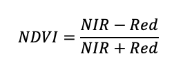
(11)
where ‘NIR’ is the near-infrared wavelength (~865 nm) and ‘Red’ correspond to red light wavelength (~665 nm). Landsat data was downloaded for each of the boundaries of the individual farms, from which images were clipped to the boundary of each field. Although data was collected from 2000 – 2021, years in which average NDVI across each field fell below 0.3 were omitted because these represent fallow years in which no crops were grown, and any productivity was due to weeds (Fig. 3).
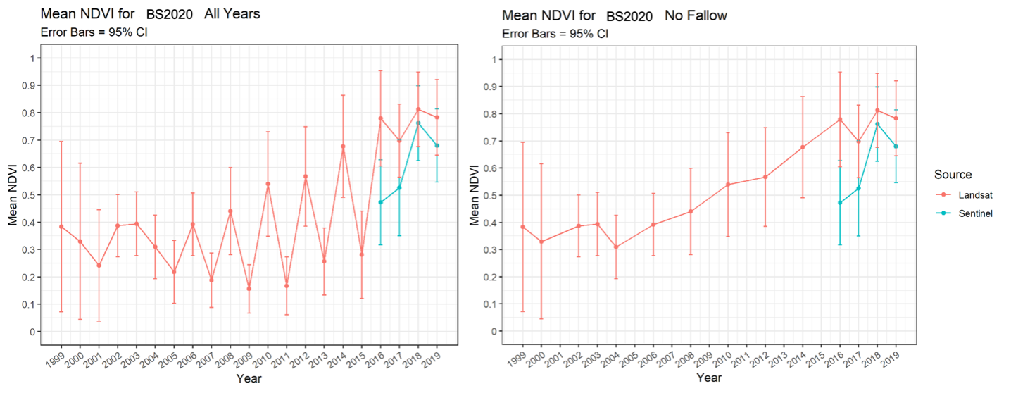
Fig. 3. Example of the data reduction process in Field 2 where fallow years were omitted based on mean NDVI across the field for a given year. Fallow years (mean NDVI < 0.3) are shown in the figure on the left, and mean NDVI without fallow years is shown on the right. While these figures show an example for one field, this process was repeated for all fields sampled.
For each field, the rasterized NDVI for each year was stacked, and WHC was classified based on each pixel’s mean and coefficient of variation (CV) to produce a single map with classifications of high, medium, and low WHC. High, medium, and low categories for mean and CV for each pixel were delineated into the three groups via the Jenks optimization method for dividing the data (Jenks, 1967). A matrix the mean and CV groups for NDVI were then derived to estimate hypothesized WHC zones (Table 7). If an area of a field is consistently productive over time, the crop is acquiring adequate water and N to maximize growth across varying annual precipitation. If the water is held in the soil, then so too is nitrate, so these areas are hypothesized to have a high WHC and a low risk of N loss. If the inverse is the case and a crop is consistently unproductive over time, the crop does not acquire enough water and N to maximize productivity under varying annual precipitation. The WHC at these points is expected to be low due to a shallow depth of fine textured soils, resulting in a high risk of N loss and low NUE.
Table 7. Classification scheme of WHC zones based on mean NDVI and the CV. Each pixel is classified based on the mean and CV across the 20 years of data collected.
|
|
Low Mean NDVI |
Medium Mean NDVI |
High Mean NDVI |
|
High CV |
Medium WHC |
Medium WHC |
Medium WHC |
|
Medium CV |
Low WHC |
Medium WHC |
Medium WHC |
|
Low CV |
Low WHC |
Medium WHC |
High WHC |
Soil samples were taken at 75 locations in each field twice per year, in March and August, randomly stratified on the classification for WHC and the experimentally varied N rates (Fig. 4). Soil samples were taken at depths of 0-15, 15-30, 30-60, 60-90, and from 90cm to as deep as possible. The depth of the deepest sample corresponded to either gravel content, rock layer or the limit of the probe (110 cm). The maximum depth at each location was recorded during sampling. Soil samples were obtained by a truck mounted hydraulic probe in March (pre-fertilization) and August (post-harvest). Soil samples were taken within 7 days prior to fertilization and within 7 days post-harvest. Winter wheat biomass samples were hand harvested in June at plant maturity at each of the sampling locations. Samples were transported in coolers on ice from the fields back to MSU where soil and plant samples were weighed wet, oven dried at 50 degree C for 7-14 days, and then weighed dry to determine water content. Plant samples were ground using an UDY Cyclone Sample Mill (UDY Corporation, Fort Collins, CO, USA). Soil samples were milled to break up peds and aggregates and sieved to remove rocks and roots to homogenize samples with a Dynacrush DC-5 soil crusher (Custom Laboratory, Hodlen, MO, USA). Aliquots were taken from each sample (plant and soil) and analyzed for total N with a combustion analyzer (Costech analytical technologies Inc., Valencia, CA, USA) in the Environmental Analytical Laboratory at MSU. Costech measurements for soil samples from March and August, Costech measurements for plant biomass samples, and as-applied N fertilizer rates were co-located by sample point, along with the derived WHC zone.
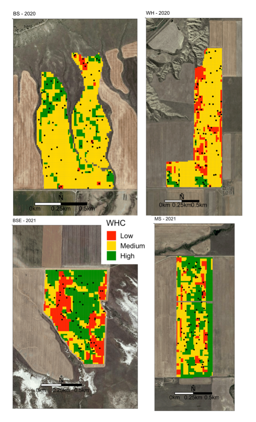
Fig. 4. Water holding capacity classifications and sampling locations for each field.
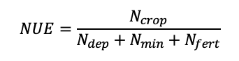
A partial mass balance approach was used to determine an estimate for efficiency for each sample location. Measured soil percent TN and bulk density were used to calculate soil TN, which was converted to kg ha-1. Crop N uptake was derived from the percent TN in the plant aboveground biomass and the closest crop yield measurement, typically a maximum distance away of 5m. Nitrogen taken up by the plant or left in the root zone after harvest were regarded as economically beneficial (efficient) uses of N because N in the crop contributes to net-return in the season the crop was grown, while N left in the root zone has the potential to be taken up by future crops and contribute to net-returns for farmers in upcoming years. However, knowledge of NUE requires knowledge about more aspects of the N cycle. Nitrogen use efficiency was estimated using soil samples prior to fertilization and post-harvest, plant biomass samples at plant maturity, and estimates of other inputs to derive the NUE. Nitrogen use efficiency was thus defined as outputs deemed efficient over the total amount of N inputs;
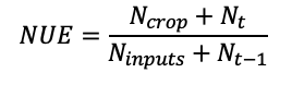
(12)
where Ncrop is N taken up by the crop measured from plant biomass samples, Nt is the amount of N in the soil after harvest measured by soil sampling, Nt-1 is the amount of N in the soil prior to N fertilizer application in the spring measured by soil sampling, and Ninputs are;
![]()
(13)
where Ndep is N deposited from the atmosphere, Nmin is mineralized N, Nfert is the inputs of N fertilizer gathered from the farmer’s as-applied N fertilizer maps, and Nfix is N fixed from the atmosphere. Due to the nature of the crop-fallow rotation there was no N fixation, so Nfix was assumed to be zero. Total N deposition was estimated to be 2.92 kg N ha-1 year-1 based on the mean total N deposition from 2000 – 2018 recorded at the closest CASTNET station at Glacier National Park (U.S. EPA, 2018). Pathways recognized in which N can be made unavailable to plants are volatilization, leaching, immobilization, runoff, and subsurface lateral flow, however the focus of this work was on quantifying how much N was partitioned to productive outputs rather than quantifying the amount of N lost via each output pathway.
However, the equation of NUE contains one unknown, the N production via mineralization within fields (Nmin). Due to the limitations of the mass balance approach measuring total N, mineralized N was modeled using a regression model derived from a review of multiple mineralization studies on the relationship between mineralization rate and percent total nitrogen (Vigil, Eghball, Cabrera, Jakubowski, & Davis, 2002);
![]()
(14)
Where Nmin is mineralized N in kg ha-1, and TN is the percent total nitrogen in the soil. Mineralization of soil organic N (SON) to plant available forms is a function of organic matter, moisture, and temperature, however equation 14 uses only percent soil total N to estimate mineralized N, introducing uncertainty into mineralized N predictions (Vigil et al., 2002). Soil organic N is typically most prevalent in the upper surface of soils, thus mineralization occurs predominately in the soil surface (Cassman & Munns, 1980). Crop N uptake is also greatest in the surface of soils due to mineralization of N and the surficial application of fertilizer N and deposition of atmospheric N. Due to most processes that contribute to NUE occurring predominately in the surface soil, only soil samples from the top 30cm were used to calculate and model NUE. A final equation for calculating NUE of the top 30cm of soil was;
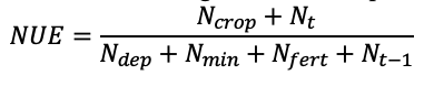
(15)
where all terms are defined above. This equation was used to calculate NUE at all 75 points within each field for both years. Sample points that did not have corresponding measurements at each depth in both March and August were omitted, yielding observations at 67, 69, 60, and 75 out of 75 sample locations in BS 2020, BSE 2021, WH 2020, and MS 2021, respectively.
NUE Modeling
To extrapolate estimates of NUE to other portions of a field and other dryland winter wheat fields, a generalizable model for estimating NUE at a subfield scale was developed with low-cost covariate data. The calculated NUE from equation 15 was the response variable used for developing a generalized model of NUE for dryland, small grain, conventionally managed Montana farms. The model intensions were to estimate subfield NUE for a given year without requiring producers to take detailed soil samples or provide parameters for complex N transport models.
Development of a general model for predicting subfield NUE relied on open source remotely sensed covariates gathered from Google Earth Engine (GEE), which were assumed to influence NUE (Table 2). All remotely sensed data were gathered from open-source GEE data repositories (Gorelick et al., 2017) and aggregated with soil sample data. Information from each covariate was extracted to each soil sample location to form the analysis dataset (Hegedus & Maxwell, 2022b; 2022c). Temporal data were gathered and delineated by year and constrained in range to the point in time that a farmer needs to make decisions on N fertilizer management of dryland winter-wheat in Montana (Hegedus & Maxwell, 2022c). Although harvest data were collected for each field, these data would not be available to make predictions at the point of a decision on N fertilizer management and were not included as covariate information for modeling NUE. The covariates selected for modeling were based on assumptions about environmental variables that influence the components of NUE and observed relationships from evaluation of observed NUE (Fig. 5). The green circles are measurements directly used to calculate NUE, besides atmospheric deposition of N. The lines leading from the green circle to NUE (blue) are thickest to illustrate the strength of the relationship between these variables and the actual NUE indicating that NUE predictions would be most accurate if these variables were measured directly. However, soil sampling is time and money intensive, so modeling NUE using data available to farmers increases a farmer’s ability to use data about their fields to make efficient management recommendations for their fields. Orange circles represent types of data relevant to each component of the calculation for NUE (green). Note that soil characteristics, topographical features, and weather all influence both mineralization of nitrogen and crop uptake at any location within a field. Grain yield and grain protein concentration are gathered from farms, but as farmers needs to make recommendations on nitrogen fertilizer in the spring prior to harvest, these data would not be available at a farmer’s decision point and not used in the model. The yield and protein circles are colored black because this data is not available, however yellow circles indicate remotely sensed covariate data that may benefit predictions of NUE (Fig. 5).
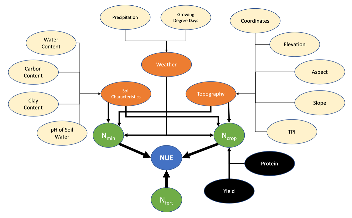
Figure 5. Conceptual model of the development of a general NUE model for Montana dryland agroecosystems. Green circles are variables that are used to directly calculate NUE, thus measuring these variables would provide the best characterization of true NUE. Orange circles are general data types that influence the components used to calculate NUE (green). Yellow circles are data types organized by general data type (orange), that are measured from remote sensing sources. The thickness of connecting arrows represents the strength of the relationship between the variable and NUE, where a variable is more directly related to NUE with thick arrows and more indirectly related with a thin arrow. The strength of a relationship between data and NUE decreases as distance between data and the blue NUE circle increases. Yield and protein would be beneficial data types for predicting crop N uptake and subsequent NUE but are not available data when a farmer models NUE to derive optimal N fertilizer rates.
A set of five candidate models were tested on their ability to predict NUE. Candidate models were chosen based on their potential for predictive and not inferential modeling. Model candidates were selected to represent simple to complex approaches with varying degrees of flexibility and assumptions. The models tested were 1) a baseline simple linear regression (SLR) model that only included as-applied nitrogen as a covariate, 2) a multiple linear regression model (MLR) using available covariates, 3) a non-linear model using an exponential decay function with as-applied N (NLR), 4) a generalized additive model (GAM), and two machine learning approaches, 5) a random forest regression model (RF) and 6) a support vector regression model (SVR). The exponential decay function was selected based on exploratory analysis of the relationship between NUE and N sources. Random forest regression is an ensemble tree approach where covariates are randomly sampled in each tree and used to classify observations (Breiman, 2001). Support vector regression maps observations to the feature space generated by the covariate data (Lau & Wu, 2008; Smola & Schölkopf, 2004).
Calculated NUE exhibits spatial dependence between neighbors, as NUE values are more similar for observations near each other than for observations with a greater distance between them. Spatial covariance structures were incorporated into the models in varying ways, from a Gaussian process spatial correlation structure used in the SLR, MLR, and NLR, (De Bastiani, Mariz de Aquino Cysneiros, Uribe-Opazo, & Galea, 2015; Diggle & Tawn, 1998; Mardia & Marshall, 1984; Xia, Ding, & Wang, 2008), a Gaussian basis function on spatial coordinates in the GAM (Gotway & Stroup, 1997; Guisan, Edwards, & Hastie, 2002; Holland, De Oliveira, Cox, & Smith, 2000; Zuur & Camphuysen, Kees, 2012), to common machine learning approaches for spatial data with the RF and SVR (Janatian et al., 2017; Langella, Basile, Bonfante, & Terribile, 2010; Walsh, Kreakie, Cantwell, & Nacci, 2017; Wang et al., 2017).
All models except the SLR and NLR were subjected to feature selection during the fitting process to optimize model performance. Top-down AIC based feature selection was performed for the MLR and GAM models, where a reduction of two AIC units with the removal of a covariate justified its omission. As AIC is not appropriate for machine learning methods, top-down RMSE based feature selection was performed for the RF and SVR models. Feature selection was based on any reduction in RMSE to determine whether withholding a covariate improved model performance. All models, except the SLR and NLR that only use as-applied N fertilizer, began feature selection with a full model that included the WHC classification, and the covariates illustrated in the yellow circles of Fig 5.
The initial candidate models were subjected to a hold-one field out cross validation approach to initially assess the ability of the model to predict NUE. Each model was independently trained on data from three out of four observed fields, and performance was tested by calculating the root-mean square error (RMSE) between the predicted and observed NUE in the withheld field (Fig. 6). The RMSE across the four test datasets were averaged for each model and compared to identify the two candidate models that generated the lowest mean RMSE. The two models selected from the hold-one field out cross validation approach were then empirically assessed using 5x2 cross validation (Dietterich, 1998). All the data from the fields were pooled and randomly split 50/50 into a training and test dataset. Both models were trained on the training dataset and RMSE was calculated based off predicted and observed NUE in the test dataset. Then the training and testing datasets were swapped (2 folds), and the process was repeated to generate four error metrics and calculate the variance of the difference in the predictions. Beginning with splitting the data 50/50, the process is repeated five times (5 folds), and the error estimates and variance from the five repetitions were used to calculate the 5x2 t-statistic (Dietterich, 1998). Assuming a t-distribution with five degrees of freedom, evidence against the null hypothesis that there was no difference in RMSE between observations and predictions from the two models was evaluated with a two-tailed significance test (α = 0.05).
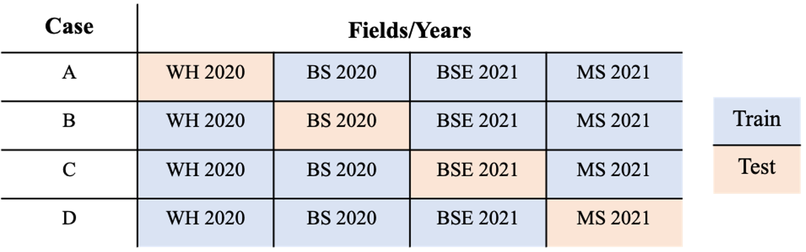
Figure 6. Hold-one field out cross validation scheme where one field is held out as a test dataset while three fields are used to train models in each of the four cases.
The final model selected for predicting NUE was used to extrapolate NUE estimates across fields per objective 3. This model was then integrated into the software package that provides users the capability to manage OFPE data, create and analyze experiments, and generate management prescriptions. This software contains the optimization model developed to generate management plans that optimize between ROI and N pollution potential. The software is presented as an open source R package with documentation guiding users how to implement the automated algorithms that receive and store farmer collected and remotely sensed data to generate the site-specific fertilizer management plans under various potential climatic and weather scenarios. The package contains methods for fitting crop responses models that characterize the ecological relationship between yield or protein and N and the environment. It also contains the predictive NUE model which is used to inform selection of optimum rates that maximize farmer profit and minimize potential for N loss. Distribution of and more information for the OFPE R-package that contains functions and algorithms written to facilitate the OFPE data workflow can be found at https://github.com/paulhegedus/OFPE.
Optimized Site-Specific N Fertilizer Rates
To derive optimized site-specific N fertilizer recommendations, field-specific models for predicting yield and protein were used in simulations to derive optimum rates under economic uncertainty. Simulation was used to develop site-specific N management that accounts for the tradeoff in net-return and NUE (SSOPT). A 10m grid was generated for each field, to which remotely sensed data were aggregated to the grid centroids to create the simulation datasets. The field-specific crop responses models trained on observed data were then used to predict grain yield and grain protein at every point in each simulated dataset for every N rate from 0 to 168 kg N ha-1 .
At every N rate for every point, the yield and protein predictions were used to calculate net-return;
![]()
(16)
where NR is the net-return ($ ha-1) received and a function of the product of the yield (kg ha-1) and the price received (P), minus the cost of the applied input (CA) multiplied by the as-applied rate of the input (AA), the fixed costs (FC) associated with production ($ ha-1) that do not include the input, and the cost per hectare of the site-specific application (ssAC). As Montana farmers receive a premium/dockage to the base price received for wheat based on grain protein concentration, the price received for calculating net-return was (Hegedus & Maxwell, 2022b; 2022c);
![]()
(17)
where P is the final price received ($ kg-1), Bp is the base price received ($ kg-1), B0pd is the intercept of the protein premium/dockage function set by the grain elevator, B1pd is the coefficient on the grain protein concentration (protein, %) and B2pd is the coefficient on the squared protein term.
In addition to simulating the net-return, NUE was predicted at every point for every N rate to account for the tradeoff in net-return and NUE. The optimum nitrogen fertilizer rate for any given point in the field was then identified as the rate that maximized profit and efficiency. Under the assumption that nitrogen use efficiency cannot exceed 100%, 1 – NUE represents the inefficient proportion of nitrogen available for crops. Desiring maximization of net-return and minimization of nitrogen use inefficiency, the optimum N fertilizer rate at each point was the rate at which the distance between net-return and nitrogen inefficiency was greatest (Fig. 7). The FFOPT net-return was based on the N rate that maximized net-return and minimized inefficiency when it was uniformly applied across the field.
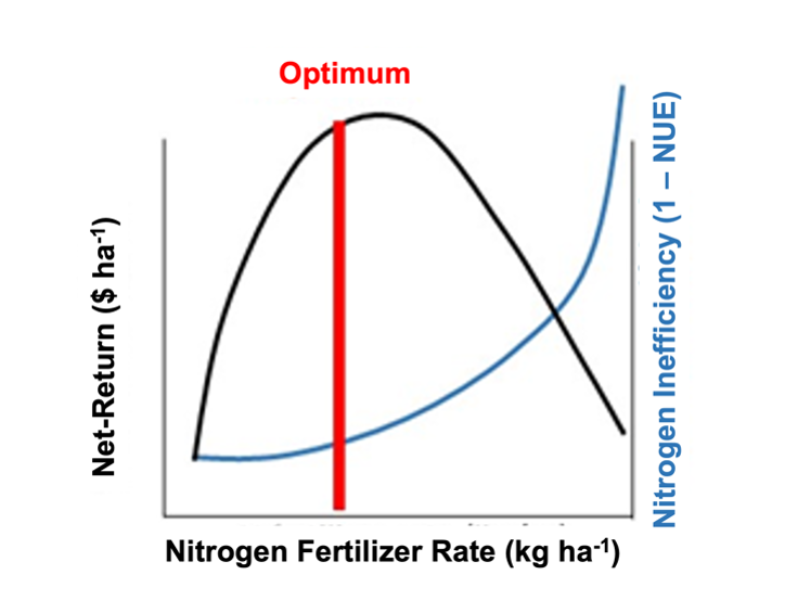
Fig. 7. Conceptual diagram of the optimization process for finding the nitrogen fertilizer rate at each point that maximizes net-return and minimizes nitrogen use inefficiency, calculated as 1 – nitrogen use efficiency.
Uncertainty in economic conditions for an upcoming year was addressed through a Monte Carlo simulation where economic conditions from previous years were randomly selected at each iteration and used to calculate net-return (Hegedus et al., 2022). Management recommendations for the SSOPT method are produced for farmers by taking the mean optimized N rates from every point in the field across the simulation. As farmers are also uncertain in the weather conditions of upcoming years, optimized N fertilizer rates were developed under four different weather conditions, where the year from 2000 – 2021 representing the most recent year OFPE was applied (Recent), most average precipitation year (Average), driest (Dry), and wet (Wet) were simulated for each field.
Crop Response Modeling
Decision support systems require models for forecasting the response of crops to variable agricultural inputs to assess management decisions when the conditions in the future year are unknown at the decision point in time. Thus, the ability of models to predict crop responses in datasets that have been held out from the model training process are vital for forecasting crop responses and expected net-return in future years. The RMSE values for grain yield, grain protein concentration, and net-return were reported for each of the five model types, for each field, and for each data split case.
The first objective was to assess the accuracy of five different types of winter wheat crop response (grain yield and grain protein concentration) forecast models using all combinations of training and holdout years (Fig. 2). The mean of the RMSE of observed and predicted grain yields were taken across the three data configurations for an average RMSE per model for each field (Table 8). These results indicate that in six out of seven fields, across any year forecasted, the RF regression resulted in the most accurate forecast of grain yield in a given test dataset with one year of data held out. Bayesian approaches were the next most accurate, where in one out of seven fields the Bayesian NLR model had the lowest RMSE out of all the model types. In two out of seven fields the Bayesian NLR had the second lowest RMSE out of all model types. Additionally, in three out of seven fields the Bayesian MLR model had the second best RMSE. The GAM was the poorest predictive model type, with the highest RMSE out of all models in five out of seven fields.
Table 8. The average RMSE of grain yield (kg ha-1) across data splits from Fig. 3. Darker shading and bolded values indicate the model type with the lowest RMSE for each field, and intermediate shading represents the second most accurate model type for forecasting crop responses in each field.
|
Field |
Beta Function |
GAM |
Bayes NLR |
Bayes MLR |
RF |
|
B1 |
2440.9090 |
5015.0961 |
2122.4399 |
2138.5884 |
2412.0508 |
|
B2 |
2645.2881 |
2149.6369 |
1883.1525 |
2068.4823 |
1797.6458 |
|
B3 |
3382.3902 |
3700.7943 |
2660.5830 |
2606.1046 |
1351.0698 |
|
D1 |
1300.2283 |
1139.2400 |
1406.4796 |
1085.3439 |
1023.4495 |
|
D2 |
1464.8009 |
3726.0322 |
1856.8694 |
2004.0815 |
1233.9528 |
|
D3 |
1333.0457 |
2123.1780 |
1521.8785 |
1537.6187 |
1187.4798 |
|
I1 |
3146.7093 |
6568.3756 |
1837.1322 |
6727.2450 |
1002.2410 |
The mean RMSE of observed and predicted grain protein concentration were calculated across the three data cases in Fig. 2 for each field (Table 9). In four out of seven fields, predictions of grain protein concentration from the RF regression had the lowest mean RMSE across data configurations and in three out of seven fields had the second lowest RMSE. The non-linear beta function had the lowest RMSE for one out of seven fields and second lowest RMSE in four out of seven fields. These results indicate that, like the RF regression models for grain yield, the RF models generated the most accurate forecasts of grain protein concentration, averaged across data configurations. On average across fields, the second-best model for forecasting grain protein concentration was the beta function. In contrast to results of grain yield models, the GAM was the best predictive model type for grain protein concentration in two out of seven fields, while the Bayesian approaches were the least accurate at forecasting protein.
Table 9. The average RMSE of grain protein concentration (%) across data splits from Fig. 3. Darker shading and bolded values indicate the model type with the lowest RMSE for each field, and intermediate shading represents the second most accurate model type for forecasting crop responses in each field.
|
Field |
Beta Function |
GAM |
Bayes NLR |
Bayes MLR |
RF |
|
B1 |
2.5005 |
3.5369 |
6.4875 |
3.7920 |
3.2084 |
|
B2 |
3.0625 |
3.7834 |
7.8040 |
3.1288 |
2.7156 |
|
B3 |
3.8652 |
1.7155 |
4.4366 |
4.8908 |
1.7377 |
|
D1 |
1.5658 |
2.0148 |
1.7419 |
2.1491 |
1.4782 |
|
D2 |
3.5321 |
4.2154 |
4.5993 |
7.3038 |
1.3496 |
|
D3 |
1.9023 |
1.3381 |
3.7526 |
2.0791 |
1.7089 |
|
I1 |
3.7393 |
11.2870 |
7.4033 |
9.5703 |
3.1114 |
When used to develop optimized site-specific N fertilizer rates, in most fields, a random forest model was used for characterizing grain yield and grain protein concentration relationships to as-applied N data (Table 10). In one field, grain yield was modeled using a modified version of a Bayesian non-linear function (Lawrence, Rew, & Maxwell, 2015) and grain protein concentration was modeled with a modified version of a non-linear sigmoid model, called the beta function (Yin, Goudriaan, Lantinga, Vos, & Spiertz, 2003). In two other fields, grain protein concentration was best predicted by a generalized additive model. Detailed description of the model types and the selection process for each field used can be found in Hegedus & Maxwell (2022b).
Table 10. Table with the best performing model type for each field, where performance was measured using repeated hold one-year out cross validation (Hegedus & Maxwell, 2022b).
|
Field |
Yield Model Type |
Protein Model Type |
|
B1 |
Bayesian Non-Linear Regression |
Non-Linear Sigmoid Function |
|
B2 |
Random Forest Regression |
Random Forest Regression |
|
B3 |
Random Forest Regression |
Generalized Additive Model |
|
D1 |
Random Forest Regression |
Random Forest Regression |
|
D2 |
Random Forest Regression |
Random Forest Regression |
|
D3 |
Random Forest Regression |
Generalized Additive Model |
|
I1 |
Random Forest Regression |
Random Forest Regression |
NUE Modeling
To make an initial assessment of efficiency common in the literature, fertilizer use efficiency was calculated and defined as;
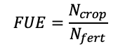
(18)
where only measured crop N uptake and as-applied N rates are used to define efficiency. Assessing the two components of this equation, an asymptotic response between crop N uptake and N fertilizer was observed (Fig. 8), indicating that as fertilizer rates increase crop N uptake is maximized and excess fertilizer has the potential to be lost from the system.
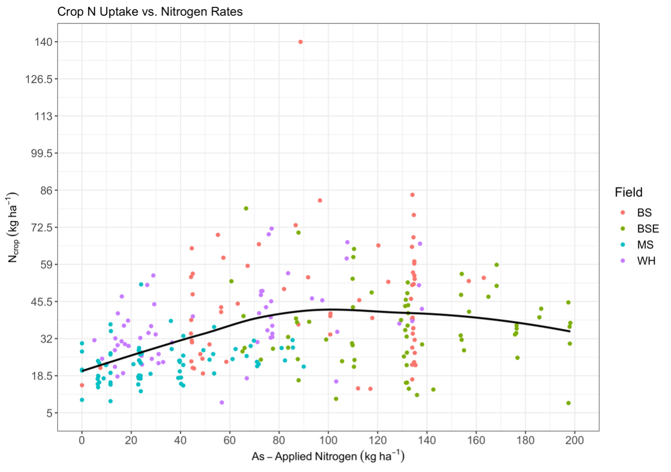
Fig. 8. Crop N uptake measured from Costech total combustion analysis of plant biomass samples vs. as-applied nitrogen measured from the farmer’s equipment. Colors represent measurements in each field and the black line shows the trend smoothed across all fields.
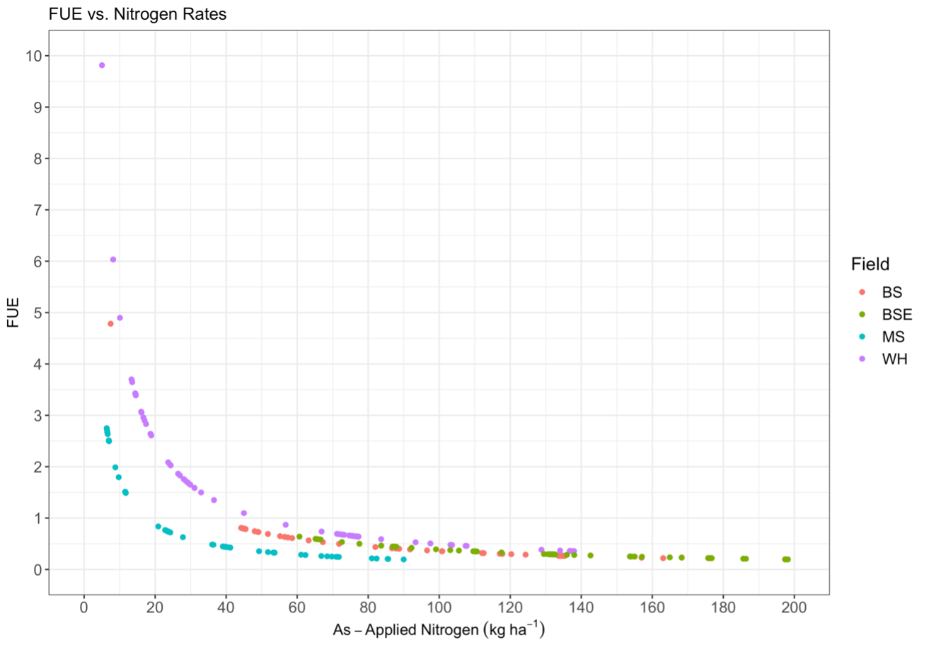
Efficiency was expected to decline with increasing N fertilizer rates due to the asymptotic nature of crop N uptake and fertilizer. A negative exponential relationship between FUE and as-applied N fertilizer was observed, where low N rate samples had the largest calculated FUE before plateauing like crop N uptake at higher N rates (Fig. 9). This indicates that while the crop uptake was low at low N fertilizer rates, the crop exceeded fertilizer inputs, indicating the presence of non-fertilizer N contributions to crop N, as expected from equation 15.
Soil total N (TN) inventories were calculated from soil TN, measured as a percent, and bulk density (g cm-3) measurements in each of the sampled layers (5 depths) at every observed point in both seasons sampled (March and August). Measured percent TN was used to estimate mineralized N (kg ha-1) at each point, for every depth interval, and in both seasons (Equation 14). Soil TN inventories, converted to kg ha-1, and mineralized N (kg ha-1) from each season were summed over the top 30cm at every point, respectively. Summed soil TN inventories from the top 30cm of soil from each sampling site from each season were used in equation 15 as Nt and Nt-1. The summed estimates of mineralized N from equation 14 using percent TN in March and August were averaged to generate a mean estimate of total mineralized N in the top 30cm at each sample point. Crop N uptake measurements were co-located via sample point and as-applied nitrogen fertilizer rates were georeferenced to each sample point. All measurements were converted to kg ha-1 and, using the constant for N deposition defined above, NUE (Equation 15) was calculated for every observed point in each field.
Efficient uses of N, crop uptake (Ncrop) and soil N in August (Nt), were highest on average in BS 2020 and BSE 2021, respectively (Table 11). With deposition (Ndep) equal, BSE 2021 had the highest average mineralization (Nmin), highest average soil N in March (Nt-1), and the highest mean experimental N fertilizer rates (Nfert) (Table 11). The higher N fertilizer rates in BSE 2021 were due to an agreement made prior to 2021 with farmer B to discontinue the use of zero N rate experimental plots. The highest mean NUE was in MS 2021 (Table 11). However, NUE rates above 1 were unexpected, as NUE is calculated as the proportion of N allocated to efficient N uses (NCrop and Nt) over the total sources of N to the system (Ndep, Nfert, Nmin, Nt-1), meaning NUE values greater than 1 indicate crop N uptake exceeded all sources of N to the soil. Explanations range from external N sources like lateral flow of N, to underestimation of mineralized N, to measurement error.
Table 11. Summary statistics for each component of NUE calculated in equation 15. Efficient uses of N are Ncrop and Ntwhile sources of N to the system are Ndep, Nfert, Nmin, and Nt-1. Efficient uses of N over sources of N are used to calculate NUE via equation 15. Note that units of N in the soil are in Mg ha-1 below, although NUE was calculated with all components in kg ha-1.
|
Ncrop (kg ha-1) |
Nt (Mg ha-1) |
Ndep (kg ha-1) |
Nfert (kg ha-1) |
Nmin (kg ha-1) |
Nt-1 (Mg ha-1) |
NUE |
|
|
BS 2020 |
|||||||
|
Min. |
13.73 |
94.84 |
2.92 |
0 |
27.55 |
102.6 |
0.59 |
|
1st Q. |
29.31 |
305.12 |
2.92 |
53.46 |
74.91 |
297.3 |
0.91 |
|
Median |
41.14 |
383.23 |
2.92 |
100.86 |
85.57 |
373.9 |
1.02 |
|
Mean |
44.56 |
354.03 |
2.92 |
95.58 |
80.12 |
352.3 |
1.01 |
|
3rd Q. |
55.28 |
419.92 |
2.92 |
134.23 |
93.18 |
423.6 |
1.12 |
|
Max. |
139.94 |
554.01 |
2.92 |
163.06 |
109.93 |
508.9 |
1.50 |
|
BSE 2021 |
|||||||
|
Min. |
8.56 |
226.4 |
2.92 |
60.64 |
48.88 |
148.1 |
0.69 |
|
1st Q. |
25.5 |
434.1 |
2.92 |
104.33 |
90.14 |
437.2 |
0.92 |
|
Median |
34.01 |
466.6 |
2.92 |
131.76 |
93.18 |
468.4 |
0.99 |
|
Mean |
35.26 |
459.2 |
2.92 |
129.43 |
91.31 |
457.1 |
1.02 |
|
3rd Q. |
43.83 |
498.1 |
2.92 |
154.58 |
96.99 |
501.6 |
1.10 |
|
Max. |
79.36 |
617.8 |
2.92 |
198.18 |
106.89 |
557.1 |
1.58 |
|
MS 2021 |
|||||||
|
Min. |
9.25 |
209.5 |
2.92 |
0 |
42.78 |
178.3 |
0.75 |
|
1st Q. |
17.97 |
417.5 |
2.92 |
11.58 |
85.57 |
426.7 |
0.95 |
|
Median |
23.05 |
483.2 |
2.92 |
23.79 |
91.66 |
460.5 |
1.03 |
|
Mean |
23.08 |
458.2 |
2.92 |
31.7 |
85.71 |
444 |
1.04 |
|
3rd Q. |
26.84 |
520.4 |
2.92 |
41.12 |
95.47 |
499.4 |
1.14 |
|
Max. |
51.72 |
739.1 |
2.92 |
89.99 |
109.93 |
647.7 |
1.41 |
|
WH 2020 |
|||||||
|
Min. |
8.76 |
129.8 |
2.92 |
5.027 |
33.65 |
136.5 |
0.51 |
|
1st Q. |
28.94 |
248 |
2.92 |
18.86 |
65.77 |
248.2 |
0.94 |
|
Median |
34.74 |
307.9 |
2.92 |
40.78 |
73.38 |
298.9 |
1.02 |
|
Mean |
37.26 |
295.1 |
2.92 |
54.93 |
70.6 |
293.4 |
1.02 |
|
3rd Q. |
45.67 |
350.3 |
2.92 |
77.03 |
81.76 |
344.8 |
1.08 |
|
Max. |
72.03 |
460.9 |
2.92 |
137.96 |
99.27 |
453.5 |
1.48 |
The soil TN measurements from March and August were not expected to significantly differ, due to the size of organic N pools in soils. Measured at the same georeferenced locations in March and August with a 1m resolution GPS, there was weak to no evidence against the null hypothesis that soil TN measurements were the same at locations in March and August in BS 2020 (t66 = -0.2516, p-value = 0.8022), weak to no evidence in WH 2020 (t59 = -0.2898, p-value = 0.773), weak to no evidence in BSE 2021 (t68 = -0.2772, p-value = 0.7824), and moderate evidence in MS 2021 (t74 = -2.0369, p-value = 0.0425). Most fields did not have statistically different soil TN between seasons, yet the total N measured in each field in March and August had a root mean square error of 58.08 Mg ha-1. While a large number, 58 Mg ha-1 is roughly 10-15% of measured soil TN, within commonly accepted uncertainty of soil N measurements.
Two potential sources of variation in measures of soil TN in March and August are differences in percent TN measured by the Costech total combustion analyzer at corresponding points in the two seasons, or differences in bulk density measurements at corresponding points in the two seasons due to measurement errors in the field. The only field in which a statistical difference between percent TN or bulk density occurred was in BS 2020, where there was strong and very strong evidence against the null hypothesis that measurements differed between March and August for percent TN (t66 = 2.488, p-value = 0.0154) and bulk density (t66 = -3.223, p-value = 0.0019), respectively. However, despite no difference observed in most fields, most measurements varied between seasons, introducing the discrepancy between total soil N between March and August. The RMSE between percent TN and bulk density were 0.0137% and 0.1399 g cm-3, indicting about 10% uncertainty between measures from the two seasons for both measures. Propagating this uncertainty to measures of soil TN in kg ha-1 yields 14% relative uncertainty in soil TN measurements.
Despite the relatively small degree of uncertainty, small changes in soil TN have a large effect on NUE calculations. Converted to kg ha-1 as used in the NUE equation, a mean discrepancy between TN in March and August (Nt and Nt-1) of up to 58,000 kg ha-1 has a large effect on calculated NUE because it washes out any difference between crop N uptake and mineralized or as-applied N, which occur on a magnitude rarely exceeding 100 kg ha-1 (Table 11). For example, if crop N uptake was 34.9 kg ha-1 and mineralized N, fertilizer N, and N deposition inputs were 70.7, 74.5, and 2.92 kg ha-1, respectively, NUE using only those components would be 0.24. However, if the soil TN in the top 30cm was 328,160.1 kg ha-1 in March and 334,414.7 kg ha-1 in August, NUE defined by equation 6 is 1.02. This calculation of NUE indicates that 6,254.6 kg ha-1 of soil TN were gained between March and August.
Based on uncertainty of soil TN measurements and the dominance of the Nt and Nt-1 on the NUE calculation, NUE was redefined as;
(19)
where all terms are defined above. This formulation calculates NUE as the ratio of N taken up by the crop to the amount of applied fertilizer N, N deposition, and estimated mineralized N. N deposition is negligible (Table 11), leaving NUE essentially a ratio of crop N to fertilizer and mineralized N. The distribution of NUE under the assumption that soil TN is invariant over time yields more realistic estimates of NUE, where WH 2020 was observed to have the highest mean NUE compared to the other fields (Table 12). The discrepancies in percent TN measurements in March and August are less influential to this calculation of NUE because estimated N mineralization was averaged at each point across the two seasons for every point. Additional uncertainty of modeling N mineralization due to the interaction between soil microbiota, moisture and temperature was recognized, but due to the importance of mineralized N in small grain agroecosystems of Montana (John et al., 2017; Sigler et al., 2018), mineralized N was retained in the final derivation of NUE (Equation 19). This equation was used to calculate NUE, referred to as the observed data in the modeling exercise below despite recognition of the uncertainties surrounding the calculation.
Table 12. Summary statistics of NUE calculated from equation 8 without soil TN for each field.
|
Field |
Minimum |
1st Quartile |
Median |
Mean |
3rd Quartile |
Maximum |
|
BS 2020 |
0.1347 |
0.1671 |
0.1956 |
0.2137 |
0.2437 |
0.3920 |
|
BSE 2021 |
0.1304 |
0.1566 |
0.1707 |
0.1790 |
0.1944 |
0.3401 |
|
MS 2021 |
0.0895 |
0.1249 |
0.1516 |
0.1556 |
0.1744 |
0.3477 |
|
WH 2020 |
0.2061 |
0.3181 |
0.4165 |
0.4341 |
0.5110 |
0.9137 |
Using the calculation of NUE defined in equation 19, a dampened negative exponential relationship between NUE and as-applied N fertilizer compared to FUE was observed (Fig. 10). The relationship was more muted for NUE than for FUE because crop N uptake did not vary across soil TN mineralized N to the denominator of the efficiency calculation decreases the proportion of crop N uptake to N inputs because mineralized N compensates for a lack of N fertilizer at low rates (Fig. 11).
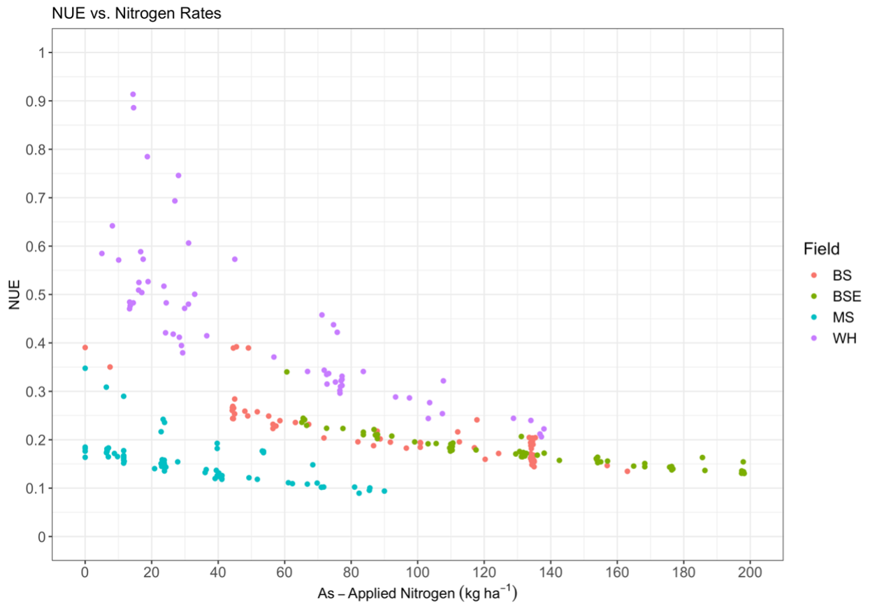
Fig. 10. Fertilizer use efficiency (NUE) vs. as-applied nitrogen measured from the farmer’s equipment. Colors represent measurements in each field.
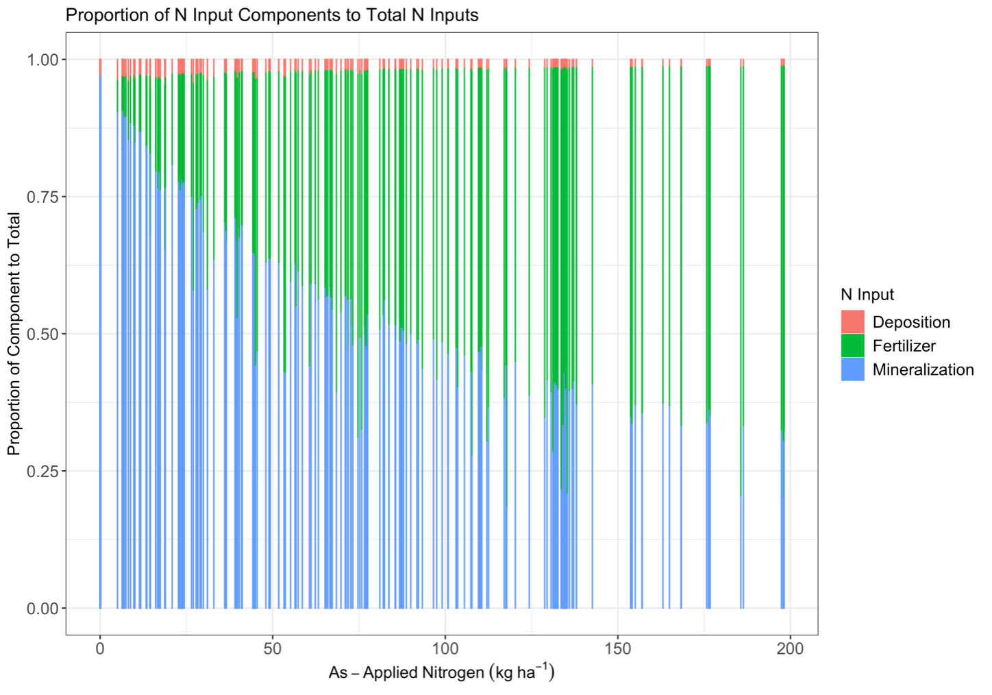
Fig. 11. The proportion of each component of N inputs to the total N inputs across N fertilizer rates. Bars are from observations across all fields.
The NUE samples were not representative of differing soil TN, thus there was no relationship between soil TN, or mineralized N which was directly calculated from soil N, and fertilizer N, indicating that mineralization was not higher or lower at low fertilizer rates compared to high fertilizer rates. However, similar to the relationship between NUE and fertilizer N, areas with low soil TN/mineralized N were also the most efficient (Fig. 12). Areas of the field with low N fertilizer or soil N, but not necessarily both, indicate places where there were low amounts of available N yet the crop was still taking up N. As mineralized N and fertilizer N increase the total amount of N inputs increases, but efficiency decreases because the crop N uptake does not increase at the same rate. While efficiency increased with a reduction of N fertilizer rates or reduction in N mineralization, low fertilizer and mineralization areas of the field do not coincide, indicating that management for NUE cannot be solely based on reducing N fertilizer rates, but requires investigating site-specific characteristics that influence N mineralization and subsequent crop N uptake.
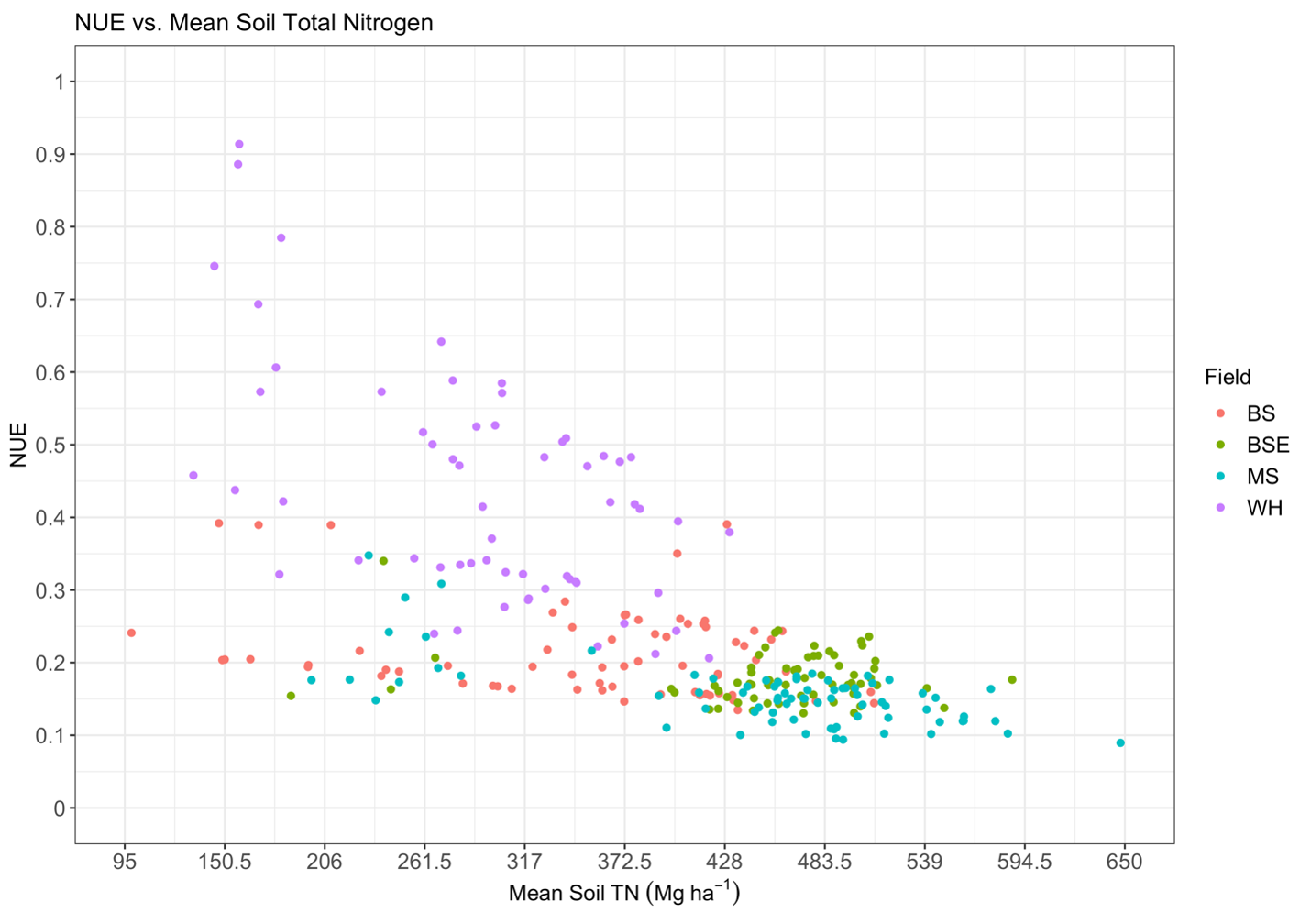
Fig. 12. The relationship of nitrogen use efficiency, calculated via equation 8, to the mean soil TN at each point. Colors indicate samples from differing fields.
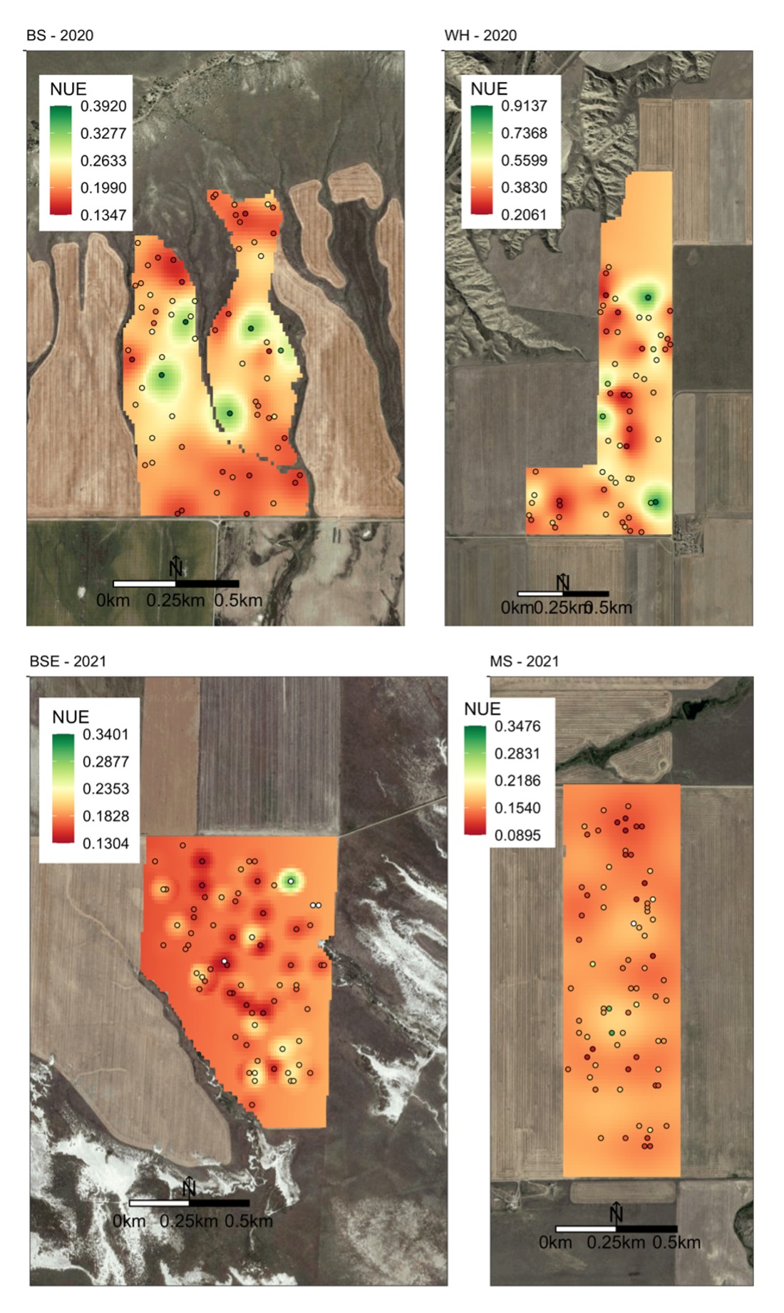
Understanding the relationships between site-specific field attributes and efficiency can lead to increases of efficiency on a subfield scale where N fertilizer rates are reduced in areas estimated to have low efficiency. Recognizing uncertainty introduced by using modeled N mineralization from observed percent TN measurements and noting it as an area of critical need in future precision agriculture research, N mineralization was retained in the final calculation of NUE for each field. The NUE calculations from measurements in each field (Fig. 13) were used as the response variable in the development of a general model for predicting subfield NUE.
The assumption guiding soil and plant biomass sampling was that areas of the field with low WHC would be more inefficient and have lower observed NUE. Results from a simple ANOVA for NUE including the interaction between WHC and field indicated no evidence of an interaction between WHC and field on NUE, but strong evidence (p < 0.01) that NUE differed between at least one pair of WHC zones and at least one pair of fields (Fig. 14). Pairwise comparisons of NUE in each group using Tukey Honest Significant Differences indicated strong evidence that NUE across all fields varied between medium and high WHC zones (p = 0.003), but little to no evidence that NUE varied between low and high or low and medium WHC zones (p > 0.1). Despite the lack of prevalent differences in NUE between WHC zones WHC was included in the list of covariates from Fig. 5 that were used to develop a general NUE model for dryland winter-wheat systems and subjected to feature selection.
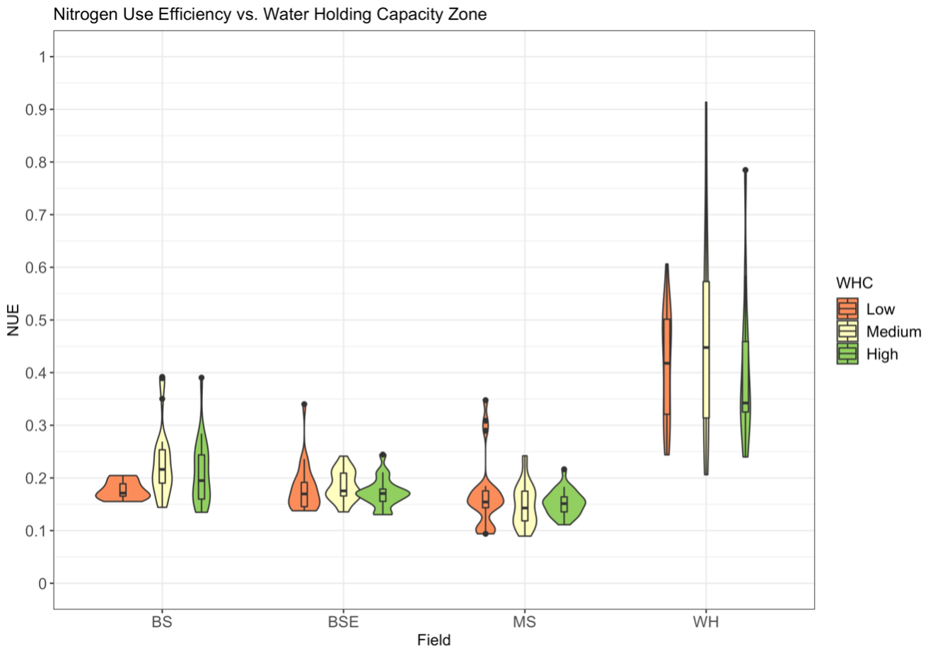
Fig. 14. Violin plot showing the distribution and frequency of NUE observations in each WHC zone for each field.
All five candidate models for NUE were tested with hold-one year out cross validation (HOOCV) illustrated in Fig. 6. The SLR had the lowest mean RMSE and the SVR had the second lowest mean RMSE, closely followed by the NLR (Table 13). However, the SLR was not the best model in any individual field, and the SVR was neither the best nor second best in any case (Table 13). The NLR model performed best for predicting NUE in two out of four withheld fields, while the MLR and GAM were best in one field each. The NLR, GAM, RF and SLR were each second best in different fields (Table 13). Based on these results, the NLR and SVR were compared by 5x2 CV to select a model, which was used in another round of 5x2 CV to compare to the SLR.
Table 13. RMSE calculated from the observed and predicted NUE from each model during the hold-one field out cross validation. Bolded values indicate the model with the lowest RMSE for a field across models and italicized values indicate the model with the second lowest RMSE for a field.
|
Test Field |
Model Tested |
|||||
|
SLR |
MLR |
NLR |
GAM |
RF |
SVR |
|
|
BS 2020 |
0.0547 |
1.0440 |
0.0338 |
0.8016 |
0.0585 |
0.0701 |
|
WH 2020 |
0.2758 |
0.4381 |
0.2718 |
0.1618 |
0.3032 |
0.3016 |
|
BSE 2021 |
0.0493 |
0.0979 |
0.0187 |
0.1762 |
0.0323 |
0.0551 |
|
MS M21 |
0.1928 |
0.1003 |
0.3069 |
0.1620 |
0.2774 |
0.1788 |
|
Mean |
0.1432 |
0.4201 |
0.1578 |
0.3254 |
0.1678 |
0.1514 |
There was strong evidence against the null hypothesis that RMSE did not differ between the NLR and SVR methods (t5 = 7.5965, p-val = 0.0006) indicating that predictions from the SVR method were significantly improved compared to the NLR. There was also strong evidence against the null hypothesis that the RMSE did not differ between the SLR and SVR methods (t5 = 9.2214, p-val = 0.0002), indicating that while the SLR had the lowest mean RMSE across fields in the HOOCV approach, the uncertainty in predictions was significantly reduced with the SVR when uncertainty due to sampling was accounted for with 5x2 CV. The SVR produced statistically better predictions compared to the NLR and SLR models, but the mean RMSE of the RF from the HOOCV approach was like the SLR, NLR, and SVR models. A final round of 5x2 CV was performed to compare predictions between the RF and SVR models to assess the two machine learning approaches. There was little to no evidence against the null hypothesis that RMSE did not differ between the RF and SVR models (t5 = 9.2214, p-val = 0.0002), and both modeled the relationship of NUE and as-applied fertilizer N well (Fig. 15). The RF was assumed to produce statistically improved predictions compared to the NLR and SLR because there was no difference between the RF and SVR, despite the SVR statistically improving predictions compared to the NLR and SLR.
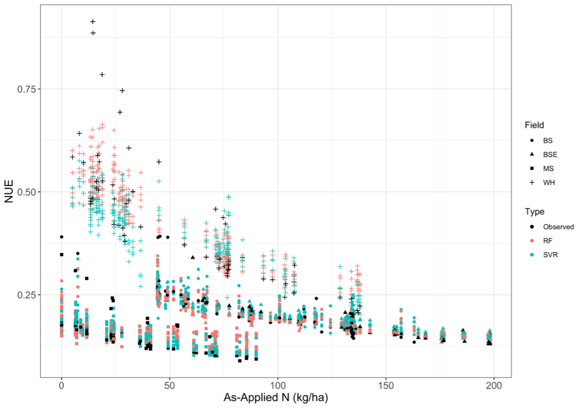
Fig. 15. Observed NUE (black points) across variable as-applied N rates, where shapes indicate each field. Predicted NUE values are RF and SVR predictions from the test sets performed in the 5x2 CV.
Although both models produced similar predictions and there was no statistical difference between the RF and SVR, the SVR was selected as the final model because the lower mean RMSE from the HOOCV analysis, which indicates that the SVR performed better than the RF when making predictions in fields unseen by the model during training. Nitrogen use efficiency predictions in each field, from SVR models trained only with data from the other three fields, tended to represent the spatial pattern of NUE calculated from observations at sample points (except in field BSE), but never captured the full range of observed NUE (Fig. 16). In most cases, NUE predictions were lower than the NUE calculated from measurements, except for in MS where the maximum predicted NUE exceeded the maximum observed NUE (Fig. 16).
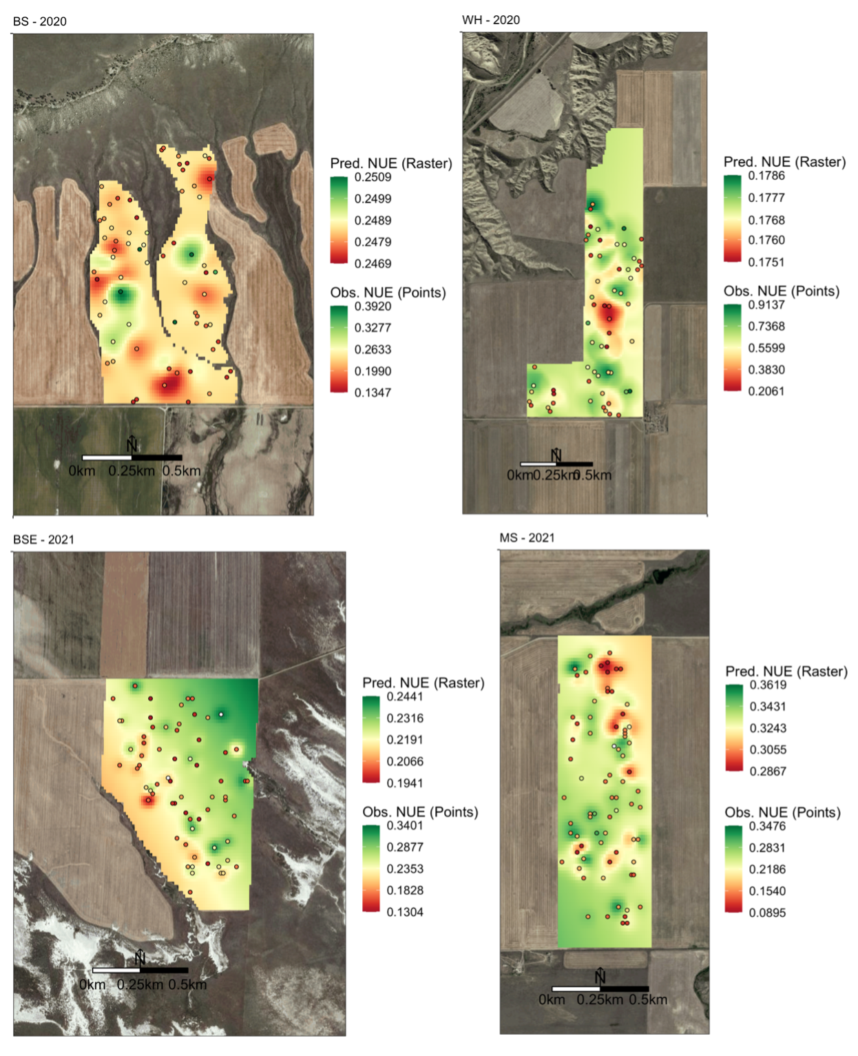
Fig. 16. Spatially interpolated predictions of NUE for each field using an SVR model trained with data from the other three fields. Points are the calculated NUE from observed soil and plant biomass measurements.
All the sampled data were compiled as a training dataset to fit a final SVR model. After top-down features selection, the SVR model that provides the best predictions of NUE using environmental and management (e.g., N fertilizer rates) covariate data (Equation 20);
![]()
(20)
Where N is the as-applied N fertilizer rate (kg ha-1), WHC is the estimated WHC zone, slope is in degrees and calculated from the USGS NED (Table 2), tpi was the topographic position index calculated from USGS NED, aspectcos was aspect in the E/W direction calculated from the USGS NED, preccy was precipitation (mm) measured from Daymet V3 (Table 2) across November 1st of the previous year to March 30th of the year samples were taken, ndvicy was the NDVI from a greenest pixel composite across Sentinel 2 images (Table 2) from January 1st to March 30th of the year samples were taken, ndvi2py is the NDVI across images from January 1st to December 31st two years prior to when samples were taken, ndwipy and ndwi2py is the median NDWI from Sentinel 2 (Table 2) across January 1st to December 31st in the year prior and two years prior to when samples were taken, respectively. Bulk density (kg m-3), derived from OpenLandMap estimates (Table 4) was bulkdensity, carboncontent was the soil organic carbon content (%) from OpenLandMap data, and phw was the pH of soil water, estimated from OpenLandMap. All covariate data were gathered from open-source data repositories or known to the farmer at the time decisions on N fertilizer needs to be made. The model was developed to predict NUE at a subfield scale under various potential N fertilizer management strategies to inform sustainable decision making by farmers in dryland winter-wheat systems of Montana.
Optimization of Site-Specific N Fertilizer Rates
Site-specific optimized N fertilizer rates were developed for each field under four simulated weather conditions. For each of the field and weather condition, the Monte Carlo simulation was performed with 100 iterations where base prices, costs of N fertilizer, and fixed costs from 2000 – 2021 were repeatedly sampled. The net-return and value of NUI was calculated for every point under every N rate for each sampled economic condition to identify the N rate that maximized profit while considering the value of N that has the potential to contribute to N pollution. While the relationship between net-return and as-applied N fertilizer varied between fields and across weather conditions, the value of NUI always increased with increasing N fertilizer rate (Fig. 17). The net-return response to variable N fertilizer rates varied between fields, yet in most fields, a similar net-return response to variable N fertilizer rates was observed across weather conditions (Fig. 17).
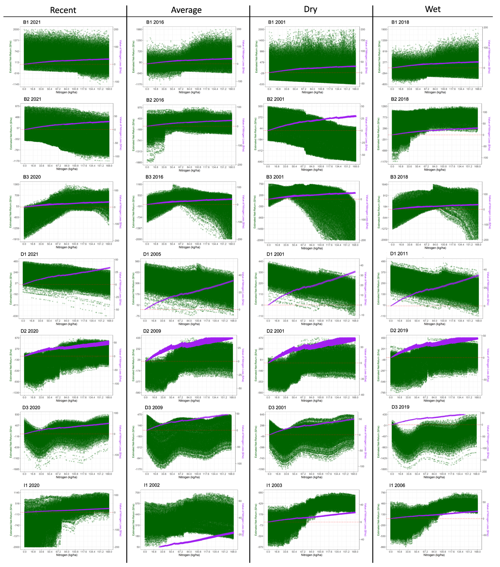
Fig. 17. Predicted net-return (left axis, green) and predicted value of nitrogen loss calculated from the nitrogen use inefficiency (right axis, purple) versus as-applied nitrogen. The distribution of points at each nitrogen rate are from predictions at that rate from every point in the field. Predictions were made using an average base price of $0.2 ha-1 and an average cost of N of $1.14 kg-1.
At every point on a 10m grid across each field where data was available to make a prediction, the value of NUI was subtracted from the net-return and the site-specific optimum N rate was identified for every iteration of the simulation for the given year simulated. The optimum N rate at every point was then averaged over the 100 repetitions to generate a site-specific N fertilizer map for each weather condition simulated for a given field (Fig. 18). Recommendations for N fertilizer rates that maximize profit and minimized the value of N loss varied across simulated years, indicating that the optimum N fertilizer rates were sensitive to varying weather conditions and in general, optimum N fertilizer rates were greatest in wet years (Fig. 18). In 3/28 fields and weather condition combinations (B2 2021, B2 2001, D1 2009), the site-specific optimized N fertilizer rate did not vary across the field, indicating that a farmer would maximize profits and NUE by applying a full-field uniform N fertilizer rate (Fig. 18). In each of those cases no fertilizer would both maximize profits and maximize NUE, and in field D1, no fertilizer was recommended in any weather condition (Fig. 18).
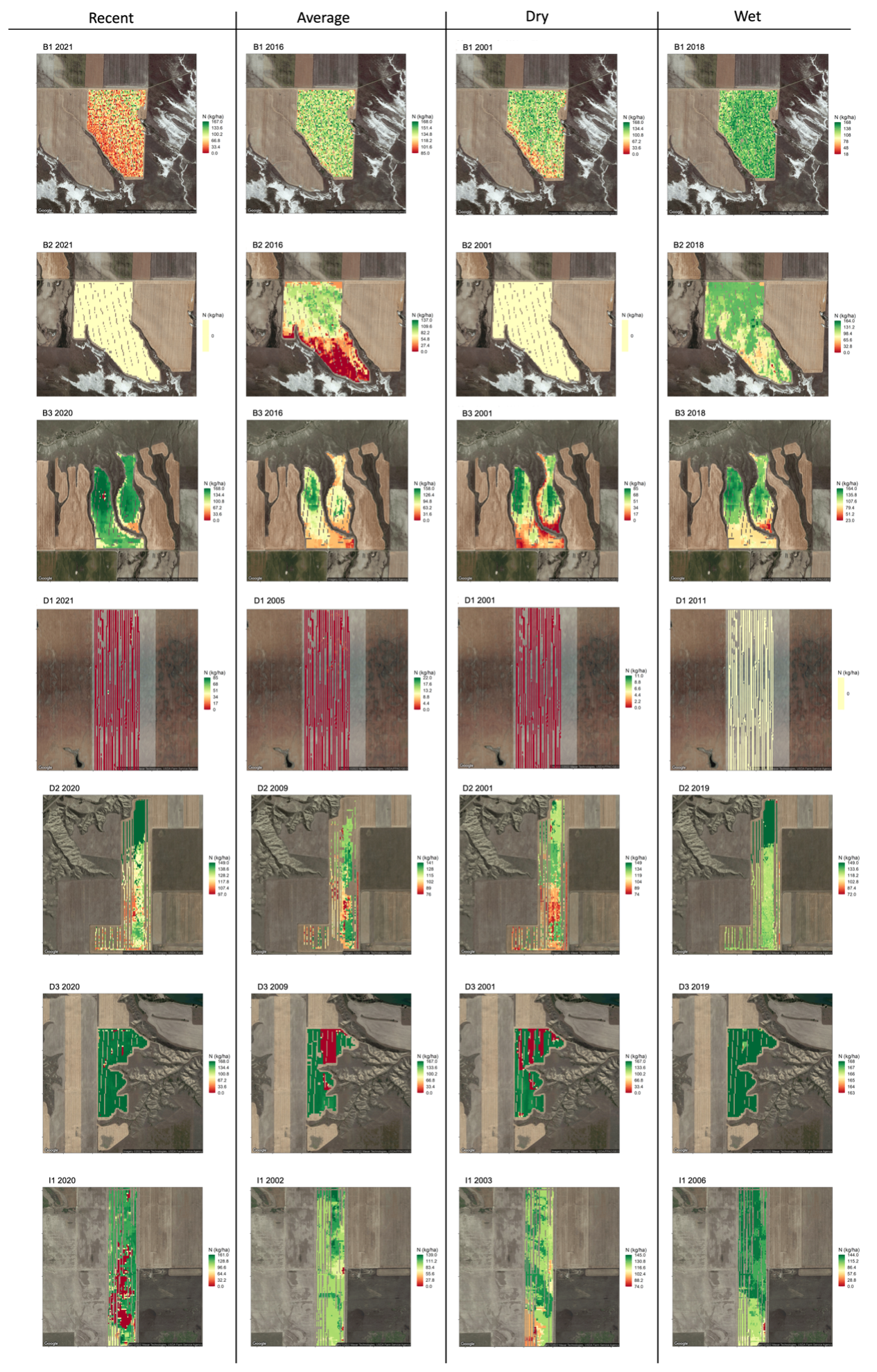
Fig. 18. Site-specific optimized nitrogen rates (kg ha-1) averaged across repetitions of the simulation for each field and weather condition.
While site-specific N fertilizer rates were generated to maximize net-return while accounting for the value of potential N inefficiency, farmers still typically lost money in some portions of their fields in all weather conditions (Fig. 19). The only field in which the farmer did not lose money anywhere across all weather conditions was field B1 (Fig. 19). Although patterns of optimized N fertilizer varied for most field between weather conditions, patterns of net-return were typically similar across weather conditions, despite changes in the magnitude of $ ha-1 (Fig. 19). Predicted net-returns tended to be lowest in dry years, with the exception of fields D2 and D3, where the farmer had the lowest net-returns in wet years (Fig. 19).
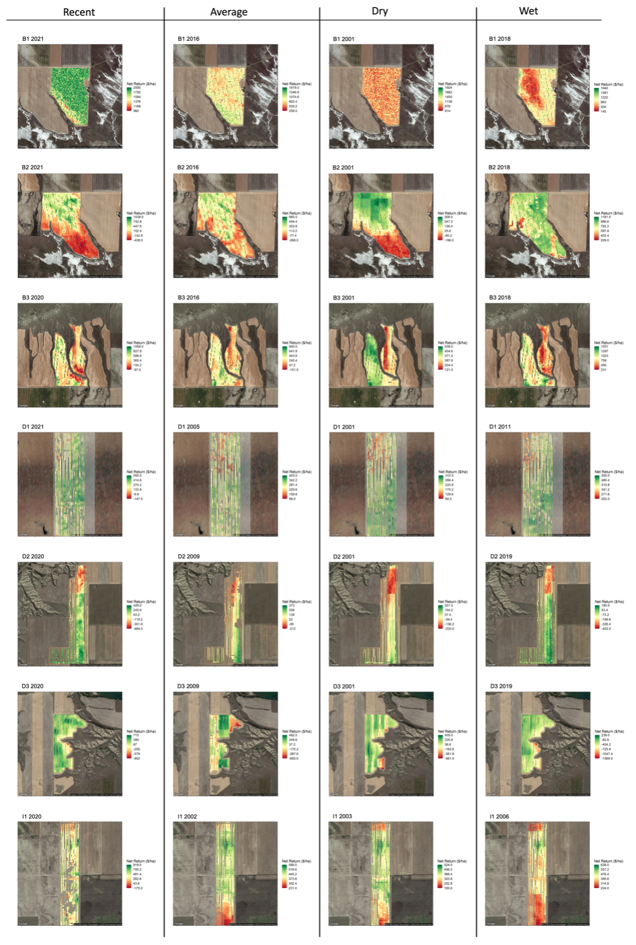
Fig. 19. Net-returns ($ kg-1) from the site-specific optimized nitrogen fertilizer strategies in Fig. 18, averaged across repetitions of the simulation for each field and weather condition.
Research outcomes
Education and Outreach
Participation summary:
A. Consultations
In late February of 2020, Paul Hegedus met with Neil Fehringer, of Fehringer Agricultural Consulting to inquire about soil sampling best practices in spring weather in Montana. The ground can be frozen into mid-March while quickly thawing and becoming muddy on a rapid diel scale, necessitating soil sampling to occur efficiently within a small-time window. Mr. Fehringer was consulted with because he is the long-term crop consultant for one of our producers, Mr. Broyles and his experience soil sampling in February and March at the field this project is conducting research. Mr. Fehringer indicated that his success soil sampling in frozen soils is due to a center mounted truck probe, leveraging the weight of the truck to push through the frozen ground, and that all operations are conducted inside of the cab. The truck mounted hydraulic soil sampling probe used for this project was mounted in the bed of a truck and thus required less than 2 inches of frozen soil. Mr. Fehringer’s services to Mr. Broyles and his operation include generating prescriptive maps for fertilizer rates. Mr. Fehringer explained that he manually adjusted fertilizer rates based on zones that were classified based off of elevation and previous yield. Paul Hegedus shared the On-Farm Precision Experiments methodology of generating fertilizer prescriptions optimized on maximum net-returns using experimental variation of fertilizer rates. Mr. Fehringer then explained his fertilizer rate trials conducted in small plots in Mr. Broyles fields, concurrent and separate from this project’s fields.
In early December of 2020, the annual Precision Agriculture Research Association (PARA) meeting was held. Due to the pandemic, it was held virtually and the list of invitees was expanded beyond those that would normally be in Great Falls for the Montana Grain Growers Conference. Included were consultants across the state, and with an attendance of 90 people, many connections were made. A handful of crop consultants stayed beyond sessions in order to discuss future collaboration and potential recruitment of clients for OFPE. Mr. Broyles’ crop consultant, Neil Fehringer, was also met with to debrief 2020 analysis results and discuss designs of 2021 trials with Mr. Broyles and his family.
In early December of 2021, the annual Precision Agriculture Research Association (PARA) meeting was held. Due to the pandemic, it was held virtually. Based on feedback from the farmers, the list of invitees was restricted to farmers, consultants, and a handful of other researchers for a total attendance of 30 people. All farmers were also met with individually to discuss results and analysis from 2021 field trials.
B. Field Days
In March of 2020, prior to fertilizer applications, soil samples were taken within each field. While Mr. Wood was unavailable, a field day at Mr. Broyles’ operation was used to demonstrate the soil sampling process using a truck mounted hydraulic probe and to explain the reasoning on gathering soil data at multiple points during the season and at such a high density. In return, the Broyles producers showed Paul Hegedus areas of the field that were accidentally burned from combine ignited fire during the prior year harvest, which were subsequently mapped. This field day was imperative to gathering information on the areas of the field that were influenced by fire, and were easily distinguishable by the fine, sooty, soil texture and lack of significant winter wheat emergence. During this visit, Mr. Broyles shared historic soil sampling and nutrient inventories, listened to the methodology for our nitrogen mass balance approach, and shared and discussed his and our expectations for the results.
In June of 2020, a second field day was conducted at the Broyles’ farm. Due to the Covid-19 pandemic, masks were worn at all times, all social distancing protocols were followed, and all Montana University System, state, and federal guidelines were adhered to. This trip was to conduct plant tissue sampling at the same locations in the field that soil samples were collected, and at the request of Mr. Broyles. There were marked differences between areas within the field that received high and low experimental fertilizer rates that Mr. Broyles requested we observed before the crop proceeded further to harvest.
Figure 1. Picture of a portion of ‘sec35mid’ taken June 25th, 2020 with 80 lbs N/acre fertilizer applied in the foreground, 0 lbs N/acre in the middle treatment, and 50 lbs N/acre beyond, below the road in the middle of the picture.
During this field day, an open discussion with the Broyles family was had about the mechanisms and timing of nitrogen uptake into the grain of the wheat plant. In addition, we were taken on a detailed tour of the experiment and shown areas of the field typically productive or unproductive, the years in which exceptions occurred, and participated in a discussion on the causes behind observations that deviated from Mr. Broyles’ historical perspective. There was no talk about site-specific fertilizing rates for net return. This producer wants the highest crop yield and protein and net return is secondary.
In March of 2021, prior to fertilizer applications, soil samples were taken within each field. Field days at Mr. Broyles’ operation were performed again to demonstrate the soil sampling process using a truck mounted hydraulic probe and to explain the reasoning on gathering soil data at multiple points during the season and at such a high density. This was also done at Mr. Merja’s field.
In June of 2021, a second field day was conducted at the Broyles’ and Merja farms. This trip was to conduct plant tissue sampling at the same locations in the field that soil samples were collected. These trips were also used as an opportunity to perform on-camera interviews with Mr. Broyles and Mr. Merja about their experiences with the OFPE project, their expectations of precision agriculture, and directions they expect the industry and science to go. These interviews will be incredibly insightful on how producers react to on-farm experimentation.
In August of 2021, after harvest, soil samples were taken within each field at Mr. Broyles and Mr. Merja’s farms to finish the sampling efforts.
C. Presentations/Publications
The first week of December is when the annual Precision Agriculture Research Association (PARA) meeting is held in Great Falls, that includes both Mr. Broyles , Mr. Wood, and Mr. Merja. At the PARA meeting, both researchers and producers have equal time to share and discuss field specific observations and results. The 2022 meeting is expected to be of interest to farmers because results from the NUE sampling and modeling effort will be shared. Throughout the grant life, 3 PARA meeting presentations have been conducted.
There are multiple papers in progress relating to this project or data collected during funding for this project. The first paper used field specific data from the farmers to justify the use of on-farm experimentation and demonstrated that the response of crops to variable N fertilizer rates not only varies within fields, but across time for a given field, and between fields in the same year, even when those fields share a border. This paper is currently under review at Agriculture, Ecosystems, and Environment. A second paper has been submitted regarding the ecological model selection process for characterizing grain yield and grain protein. The results of this paper showed that the most appropriate model form for crop responses varies between fields and is sensitive to the years used in training datasets. This paper is in review at Precision Agriculture. A third paper is also in review at Precision Agriculture that assesses the benefit of including covariate data gathered up to the point that a decision on N fertilizer management must be made. The results of this paper indicate that including data up to a decision point when training ecological crop response models benefits decision making by increasing prediction accuracy. Evaluation of NUE and development of a generalizable NUE model is currently in preparation for submission to an academic journal. Finally, demonstration of the optimization of N fertilizer rates based on maximized net-return and minimized potential for N loss is being prepared for submission to Precision Agriculture.
D. Fact Sheets/Conferences
In addition to publications in academic journals, a MontGuide is in preparation that describes the methods and benefits of applying site-specific N fertilizer management. This fact sheet will be disseminated through the Montana State University Extension service. Additionally, results from this project have been presented at the Ecological Society of American in 2020, the Montana Organic Association annual conference in 2021, and will be presented at the International Conference of Precision Agriculture in 2022.