Final report for GW19-198
Project Information
The world population is growing and food needs continue to rise. All the while agricultural practices of high inputs and vast continuous monocultures are degrading land, waterways, and reducing ecological services worldwide. Organic agriculture proposes partial solutions to these problems by reducing inputs and emphasizing soil health, but it is unable to match conventional agriculture yields. Conventional systems have been able to increase yields with the adoption of precision agricultural (PA) techniques; techniques that allow variable rates of nitrogen to be applied to specific field points to maximize yield and reduce nitrogen runoff. A similar approach could be adopted in organic systems by mapping yields and optimizing seed rates of both nitrogen-fixing green manures, and cash crops that follow, to maximize yields of the cash crops. By optimizing seeding rates to meet the variability within each of their fields, organic farmers could reduce their costs, increase their plant-available nitrogen levels, and see improved crop output both in yield and quality. Thus, I propose to use newly developed PA tools and adapt them to organic production systems much the same way as synthetic fertilizer applications have been optimized. Organic systems have unique variables relative to conventional systems such as plant nutrient availability and weed density. To explore these sources of variability in cash crop responses, the field trials will be used to develop crop yield predictive models to examine long-term resilience in organic grain rotations. Findings will be shared with both the organic and conventional communities who see benefits to using green manures and varying seeding rates in both cover and cash crops. This research will provide farmers with new on-farm experimentation methodologies and access to modern data sources to increase understanding of what variables cause variation in crop response across their fields and can be managed to increase their sustainability.
Overall my objectives seek to increase resilience and thereby sustainability and profitability of organic farms by gaining an understanding of within-field spatial variability in factors driving crop response and providing algorithms that will allow optimized site-specific best organic management practices.
1. Determine the first-principle relationship between green manure (GM) crop seeding rate nitrogen left in the soil and following kamut crop growth over a range of kamut seeding rates.
2. Establish OFPEs on three farms with one or two fields each, where GM seeding rate will be site-specifically varied and subsequent year cereal crop seeding rate factorially varied to determine the influence of seeding rates of successive crops on cereal crop yield and grain protein content. Simultaneously monitor weed densities and determine their influence on crop response. One additional farm with two fields will vary bloodmeal rates, an organic nitrogen input, as they do not use green manure as a nitrogen source.
3. Develop models to predict optimal site-specific GM seeding rates and following year cereal crop seeding rates to maximize producer profitability in the organic fields where OFPE is applied.
4. Share the results of the research in a range of venues.
Table 1 – Gantt Chart – Project Timeline

Table 1 shows the projected timeline for each objective of the project. The Greenhouse study (Obj. 1) will be conducted first to provide information for the field experiments. The model (Obj. 3) will be built simultaneously and updated as new information from the field experiments (Obj. 2) becomes available. The two field growing seasons, the cornerstone experiments of the project, are highlighted under objective 2.
Cooperators
- - Producer
Research
Objective 1) Greenhouse Experiment
The goal of this experiment was to determine optimum green manure (GM) seeding rates to maximize biomass production and following kamut (Triticum turanicum) yield as a result of nitrogen fixed by the GM and made available to kamut. Garden boxes measuring 50cm by 50cm and 25cm deep were filled with sterilized soil mixed with 50% sand in order to better emulate low nitrogen and sandy conditions typical of agricultural settings in north central Montana. The green manure tested was Arvika green peas, a common Montana crop and variety. Inoculated seeds were planted 3cm deep in rows 16cm apart; similar to how they would be planted in field conditions. Seeding rates encompassed a range well below and above typical farmer chosen rates and included pea rates at 0, 42, 78, 204, and 486 kg/ha (0, 7, 13, 34, and 81 seeds (150mg each) per box). Pea plants were grown for approximately eight weeks at optimal light and temperature growth conditions. Plants were terminated at first flowering stage, when roughly half the plants were flowering, which is the recommended termination stage to maximize N production and minimize water loss in arid conditions (McCauley et al., 2012). At termination, a subset of plants was collected, dried, and weighed to estimate biomass of the remaining plants which were incorporated into the soil. Pea plants were mixed into the soil and allowed to decompose over six weeks; soil was kept moist and occasionally stirred with a shovel.
Kamut seed was planted into the boxes at four different rates: 25, 50, 75, 100 seeds/box (30, 60, 90, 120 kg/ha). Each kamut rate was planted across each pea rate to create a full factorial design. Kamut was grown until maturity, which took approximately twelve weeks, then each head was harvested and weighed to determine crop yield by plant and by box. Soil was sampled to track nitrogen gain and loss in the soil at multiple time points: at pea planting, pea termination, kamut planting, and again following kamut harvest. An experimental oversight was noted in that pea seeds themselves contain approximately 4% nitrogen (personal communication, Perry Miller, 2022). The highest rate of pea seeding rate therefore saw an increase in nitrogen availability despite significantly reduced plant growth due to competition. Because we were seeking to understand how nitrogen fixation would be affected by plant densities, this top rate (which is well above any recommended seeding rate), was dropped from most of the analyses and the figures shown in results. When only nitrogen change in the soil was assessed we could still use these data points by accounting for the nitrogen added to the soil via the seeds themselves. Data was analyzed with regression analysis using generalized linear models to determine the relationship between GM seeding rate and kamut seeding rate and final kamut biomass and yield response.
Objective 2) On Farm Precision Experimentation of Seeding Rates and Harvest Yield
In this project on farm precision experimentation (OFPE) was used to adaptively manage inputs on organic farms. OFPE was used to optimize seeding rates of nitrogen-fixing GM crops, and non-GM cash crops such as wheat, barley, or kamut, and on one farm bloodmeal was varied to determine its optimum input rate. Rates were varied randomly across the field in order to understand within field spatial variation based on continuous georeferenced yield and protein monitor combine data. As all organic farmers face weed challenges, variation in weed density was mapped using a range of methods (Maxwell et al., 2005).
A total of four separate Montana certified organic farms collaborated on this project, and each farm conducted experiments on at least one field. Farmer collaborators include Bob Quinn and Seth Goodman, Casey Bailey, Ole Norgaard, and Ty O’Connor. To maintain anonymity farms henceforth are simply referred to, in no particular order, as farms A:D. Farm A is near Big Sandy, farm B near Fort Benton, farm C near Shonkin, and finally farm D near Ekalaka. The first three farms conducted OFPE with seeding rates of GMs and cash crops, and farm D experimented with varied rates of bloodmeal, an organically approved source of nitrogen, on wheat cash crops. The acreages of the fields vary from 32 to 93 hectares.
Initially one field per farm was extensively soil sampled (approximately one sample for every two acres). Farm B and farm D added a second field to the experimentation and these fields were not soil sampled due to cost restrictions. The samples were analyzed for nitrogen content in Montana State University’s Environmental Analytics Laboratory (EAL) and were used to build a fertility map of each field. Wherever possible, the fertility map, previous yields, and other geographic variables were used to stratify GM seeding rate strips across the field to maximize variability within each randomized replicated strip.
Experiments were initially designed to incorporate five rates of pea at 0X, 1.5X, 1.0X, 0.75X, and 0.5X farmer selected rates, these were to be planted with standard planters owned by each farmer. Given differences in equipment and ever-changing field and weather conditions the exact number and level of different rates was not followed precisely. In year two, differing seed rates of cereal crop were to be planted on top of the GM variable strips such that each GM rate will have every level of the cereal crop overlaid. Cereal seed rates were to similarly be 1.25X, 1.0X, 0.75X, and 0.5X of recommended organic rates. These were guidelines, and in practice rates were adjusted by farmers’ specific needs as seen below.
The farms joined the project at different times and experiments therefore started in different years. In 2019 farmer A planted peas on a 32 hectare field (soil sampled) at rates of 0, 60, 90, and 120kg/ha, and tilled them in after approximately eight weeks. In 2020 they planted barley over the same field at 60, 90, and 120 kg/ha, unfortunately a storm caused hail damage that wiped out 90% of the crop, and the remaining plant matter was removed as hay bales. Barley was again planted at the same rates as in 2020 in the spring of 2021, and harvested at the end of July 2021. In 2019 farmer B planted winter wheat at 60, 90, and 120 kg/ha across a 40 hectare field site (soil sampled); this field was severely wind damaged to the point where spring wheat was reseeded in a patchwork that made yield data collection based on seeding rate variation meaningless. In spring they also planted peas at 70, 90, 110, 130 kg/ha on a different 32 hectare field (not soil sampled), and planted winter wheat in fall 2020. The farmer chose not to vary the winter wheat seeding rates, but the experiment still provided important data on the effects of the varied pea rates. In spring 2020 farmer C planted peas at rates of 80, 100, 120, and 140 kg/ha across a 93 hectare field (soil sampled) and tilled them in approximately eight weeks later. Winter wheat was planted in fall 2020 across the field at varied rates of 55, 70, 85, and 100 kg/ha. Farmer D planted spring wheat at a uniform rate across a 32 hectare field (soil sampled) and a 67 hectare field (not soil sampled). Bloodmeal was applied across both fields at nitrogen rates of 0, 3.5, 7, 15, 20 kg/ha. Yield data were collected from the combine monitors. Farmer D was set to repeat this experiment in 2021 however suffered severe crop loss across their farm due to drought. The other three farms reported harvest data from cereal crops after harvest in late summer 2021.
Crop and weed data were collected during the growing season to track how the different seeding rates affected crop and weed growth. Approximately 60 points were chosen at random across each field, and stratified on seeding rate, in order to non-destructively survey plant growth. A wire frame with an area of 0.25m2 was placed on the ground at the point and two researchers viewed its contents to estimate crop and weed cover. Each researcher estimated the amount of crop canopy coverage in the circle from 0 to 100 percent. To reduce bias the researchers then shared their numbers and recorded the average. The height of an average looking crop plant was then also recorded, and the percent cover and height was multiplied in order to estimate the volume that the crop occupies. Finally, several crop plants were measured, then collected and dried to create a regression of plant volume to biomass in order to convert plant volumes into estimates of plant biomass. This method was additionally conducted for the three most dominant weed species within the wire frame at each of the points across the field. Each species can have up to a total of 100% canopy cover. To further verify seeding rate affect across the field, crop counts were collected from across the field to determine germination rate and actual plant number within each seeding rate across the field.
Each farmer used their own field equipment, thus dimensions of experimental strips for each farm were slightly different depending on width of seeder and combine. GPS units on tractors and combines, and geospatially referenced yield monitors on the combines were already in place on the farmer’s equipment. Automatically aggregated data for each field includes as-applied maps of variable seeding rates, yield points, NDVI, and topographic information (elevation, slope, aspect). As-applied maps were collected from the seeder computer, yield points were collected from combine mounted yield monitors, and NDVI and topographic information were compiled via google earth engine of satellite information from NASA’s Modis and Landsat 8 instruments (He et al., 2018). Data were analyzed using linear and non-linear regression and random forest with R statistics packages in R Studio (Version 1.1.453 – © 2009-2018 RStudio, Inc.). Maps for producers and other reports including this one were produced in QGIS, and R Studio.
Modeling:
A data framework, already functioning in our lab for nitrogen fertilizer optimization across whole fields in conventional systems, was adjusted and updated for organic agriculture . The current R package that our lab has developed to produce an economic comparison among different nitrogen fertilizer management strategies (e.g. site-specific variable rate, no fertilizer, uniform farmer selected rate, uniform optimum rate, and organic with no fertilizer) was updated to compare site-specific variable GM seeding rate, no GM (tillage based fallow), uniform farmer selected GM seeding rate, and optimum uniform GM seeding rate based on farmer net return (https://paulhegedus.github.io/OFPE-Website/).
Statistical Analysis:
Point data from the seeder (as applied map) and combine (yield map) were added to a square 10m x 10m grid of the field. Means of points were taken when more than one point existed per cell. To remove border effects, headlands, as measured by 30 m from the field edge, were removed from analysis. From this accumulated data set random forest models were constructed to find optimized seeding rates for minimized weed presence and maximized yield. Moran’s I test, linear models and random forest models were tested in R, on data sets assembled in QGIS. Moran’s I test was used to verify that the seeding rate variable interacted spatially and affected weeds and yields differently in different parts of the field. Likely variables to be included in random forest models were verified using R package Boruta (Kursa and Rudniki, 2010). The random forest model used for each field varied based on input data, but a typical model is shown below in equation one.
[Equation 1] Yield ~ pea_SR, barley_SR, elevation, x, y, slope, aspect, TPI, weed2019, weed2020, weed2021, NDVI2py, NDVIpy, NDVIcy, precipCY, sat_bulkdensity, sat_clay, sat_pH, sat_water, sat_carbon, nitrate6, nitrate24
The random forest model seen above included yield as the response variable to seeding rate of pea and wheat, and topographic variables: elevation, x and y coordinate points, slope, aspect, and Topographic Position Index (TPI); the season’s weed values as found from interpolated sample data; satellite data including: Normalized Difference Vegetation Index (NDVI) from the harvest year, the year prior to harvest, and two years prior to harvest, the current year precipitation, bulk density, clay content, pH, water content, and soil carbon; and soil sample data including: nitrate to six inches, and nitrate to 24 inches. Based on the predictions of this model ideal seeding rates were estimated for maximized yield across each grid cell. As an example, a subset of the variables collected for the above method is shown in maps in Figure 1 including topographic variables (1A), satellite variables (1B), manually sampled variables (1C), and machine variables (1D).
Economic Analysis:
Net returns were calculated based on farmers’ stated costs of seed and price received for product. Prices received in our tested harvest years ranged from $13 a bushel to $23 a bushel. To compare these to historic conditions a data set tracking organic prices (received from elevators) over the last twenty years was used, we also included varied fixed rates over these years as collected from USDA (see table 1). To ascertain the probability that one method would outcompete another, a Monte Carlo simulation analysis was conducted using the twenty years of economic data such that the simulation outcome of yield and recommended seeding rates was tested across every year of economic data. In this way we state the probability that one method (farmer chosen rates, optimum average rates, or variable seeding rate) is better than the others given varied economic conditions.
Table 1: Twenty years of economic data collected from local Montana elevators from 2000-2021.
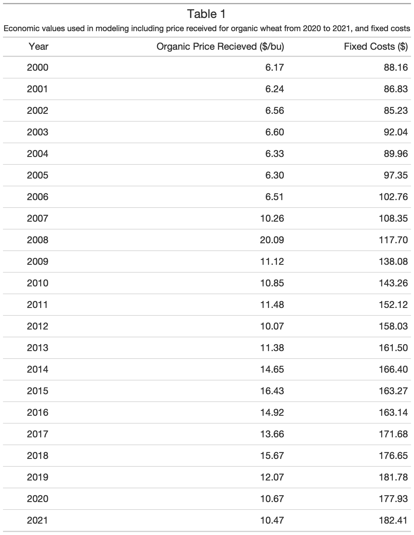
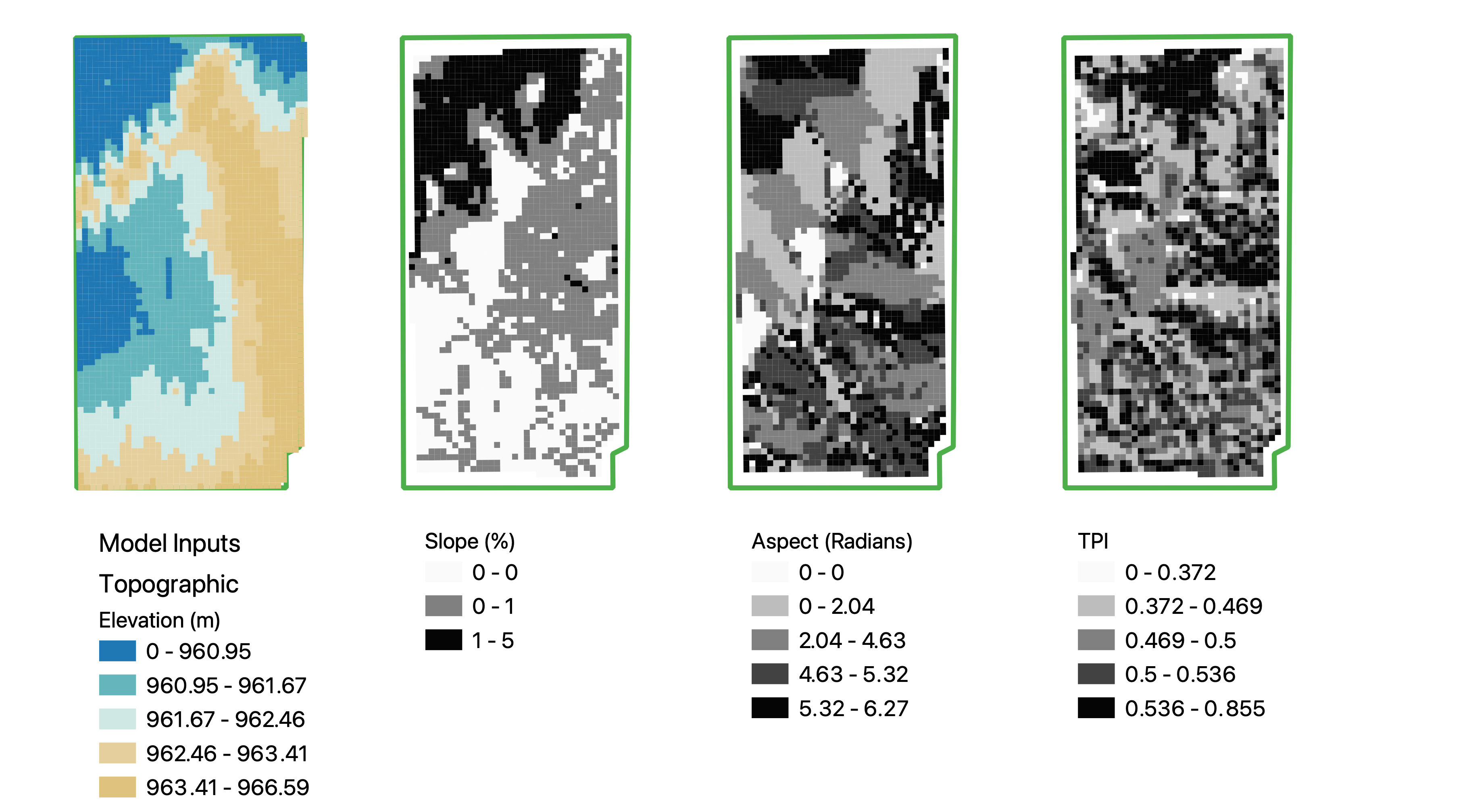
Figure 1A – 80 acre On Farm Precision Experimentation Field showing topographic input variables for modeling including panel 1) elevation, panel 2) slope, panel 3) aspect, and panel 4) topographic position index (TPI).
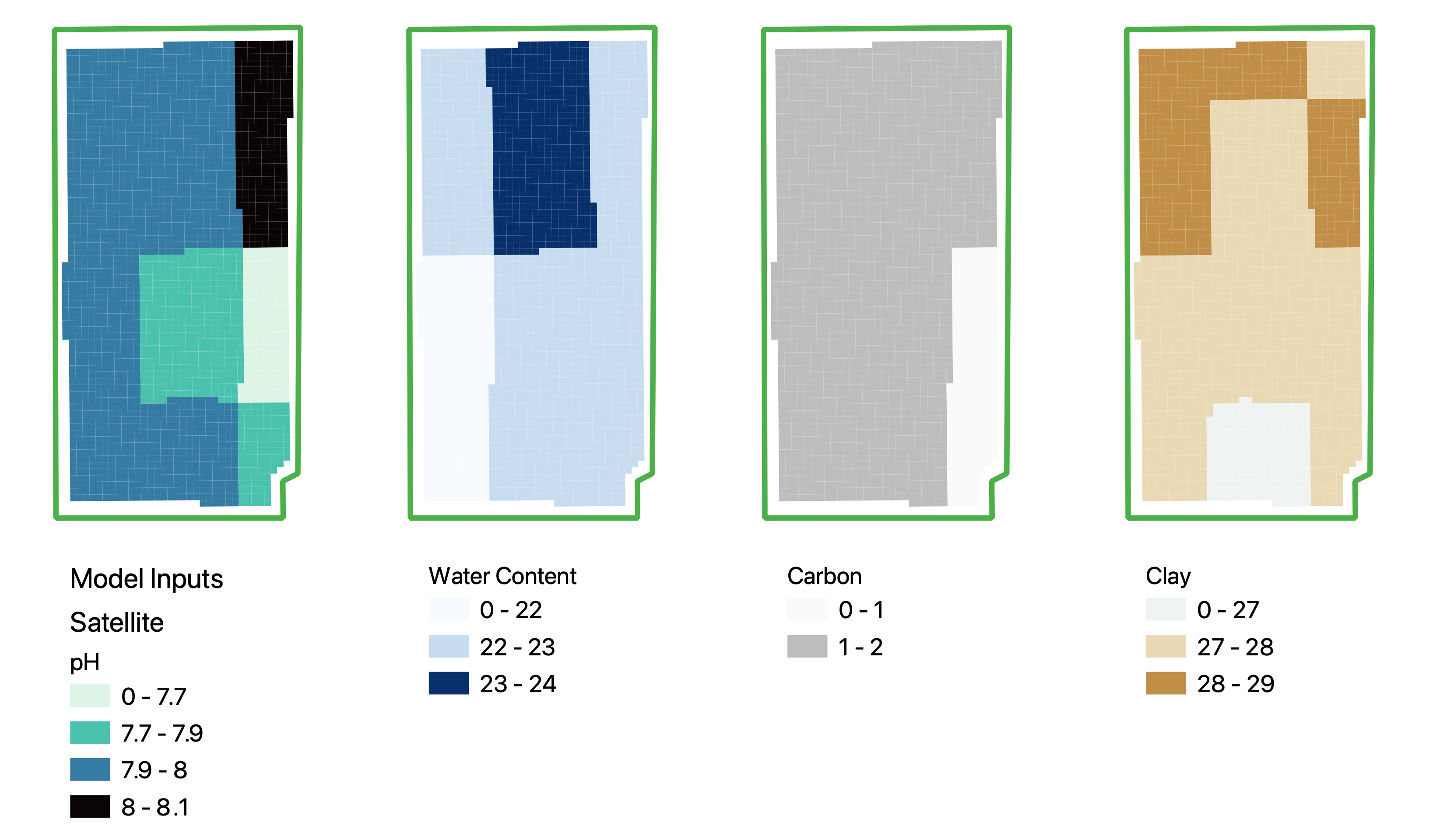
Figure 1B – 80 acre On Farm Precision Experimentation Field showing satellite input variables for modeling including panel 1) pH, panel 2) water content, panel 3) carbon content (%), and panel 4) clay content (%).
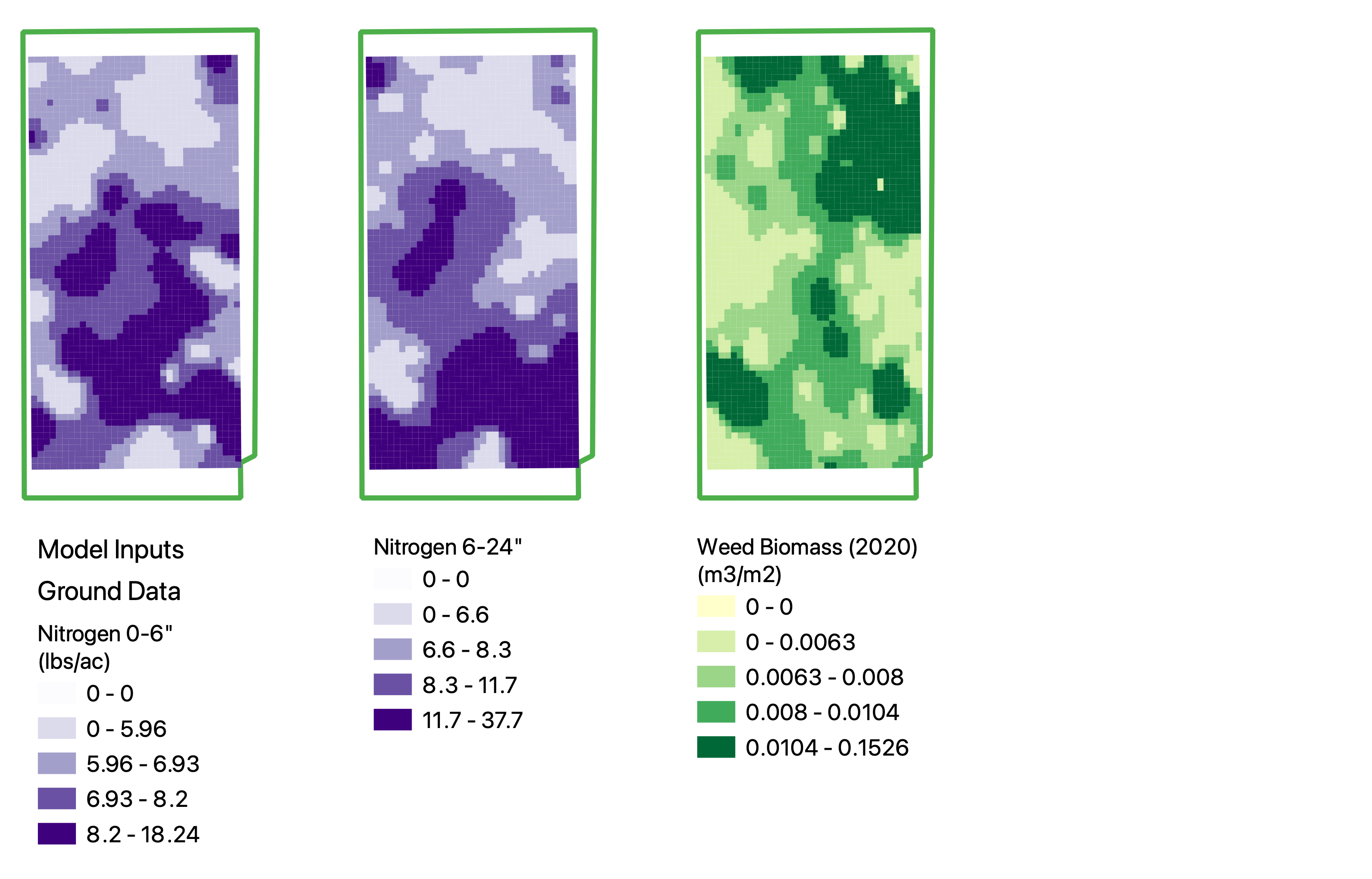
Figure 1C – 80 acre On Farm Precision Experimentation Field showing on the ground collected data for modeling including panel 1) nitrate 0-6”, panel 2) nitrate 6-24”, and panel 3) sampled weed biomass in cubic meters per square meter.
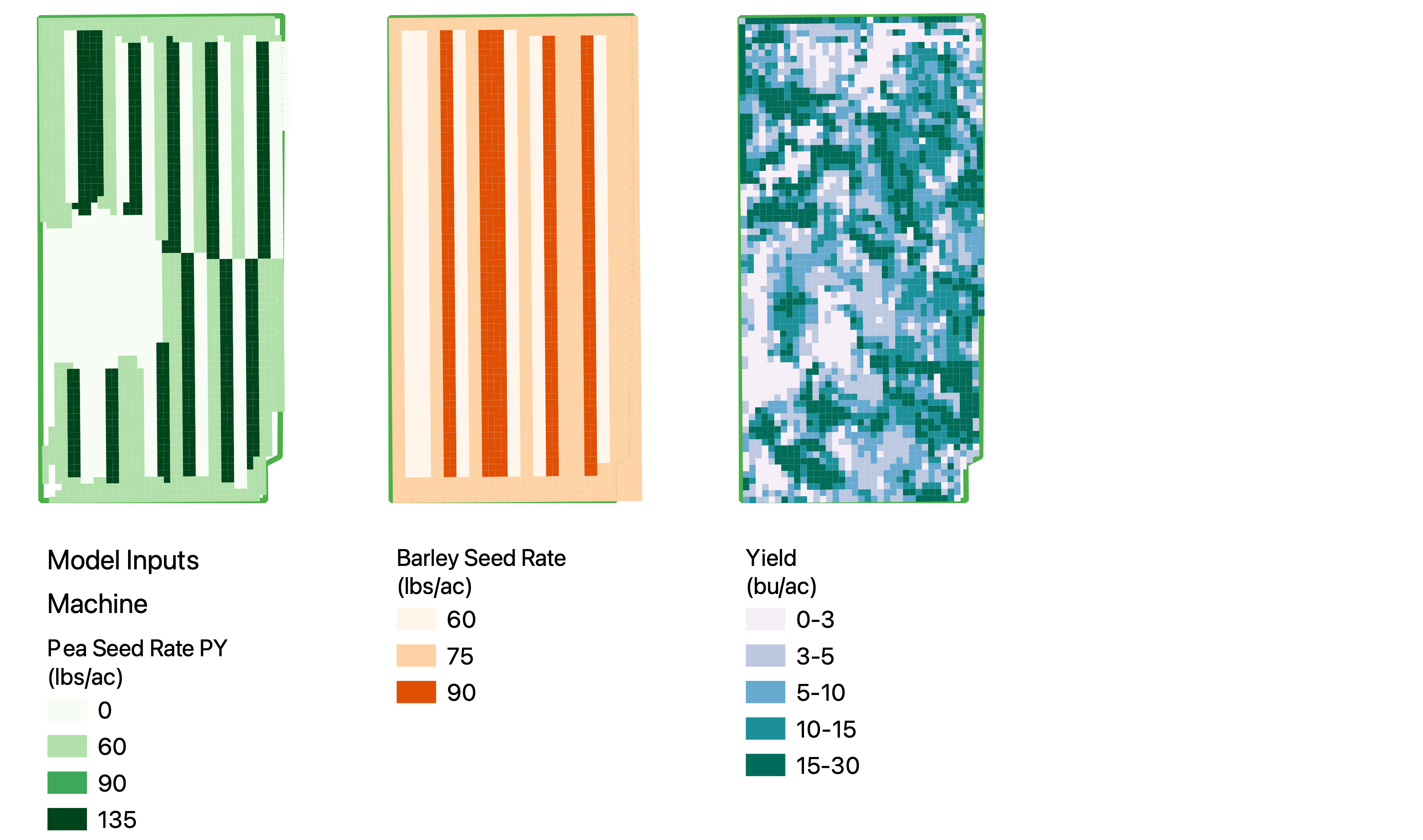
Figure 1D – 80 acre On Farm Precision Experimentation Field showing on the machine collected data for modeling including panel 1) experimental pea seeding rates from 2019, panel 2) experimental barley seeding rates from 2020 (repeated in 2021 due to hail 2020), and panel 3) combine yield results from barley harvest 2021.
Objective 3) Computer Model and App
A data framework, already functioning in our lab for nitrogen fertilizer optimization across whole fields in conventional systems, was adjusted and updated for organic agriculture . The current R package that our lab has developed to produce an economic comparison among different nitrogen fertilizer management strategies (e.g. site-specific variable rate, no fertilizer, uniform farmer selected rate, uniform optimum rate, and organic with no fertilizer) was updated to compare site-specific variable GM seeding rate, no GM (tillage based fallow), uniform farmer selected GM seeding rate, and optimum uniform GM seeding rate based on farmer net return (https://paulhegedus.github.io/OFPE-Website/). The model compares different wheat seeding rates on top of each of the GM seeding rate strategies (Figure 1 under Methods). A final output of the model generates a profit maximizing site-specific GM seeding rate and wheat seeding rate map (Figure 2 under Results). This study is intended to be the beginning of a much longer study, as the predictive power of an OFPE based model increases over time. Crucial to the long term implementation of this methodology is automation of OFPE and minimizing farmer knowledgebase and time commitment required to apply OFPE results (https://sites.google.com/site/ofpeframework/home). The longer study will maintain GM and wheat seeding rate experimentation, and incorporate any other input experiments farmers are interested in pursuing.
All code is part of a package built in the R language and environment. The first step in producing experimental maps for farmers was to access a communal lab database. Within this database historical spatial data was stored including: farm boundaries and field boundaries, yield and protein data from combine monitors, and any experimental input rates from sprayers, spreaders, and seeders. Many other data types for each field are also freely collected via Google Earth Engine comprising topographical information including slope, aspect, and topographic position index, weather data including precipitation, and growing degree days, vegetation indices including NDVI, NDRE, and CIRE, and soil moisture from SSURGO. A script built in R was used to aggregate data from the database for a particular field. The aggregated data include: field name, farmer name, spatial coordinates, previous experimental year yield, previous experimental year seeding rate, topographic information, current year precipitation up to March 1 (point of decision making), precipitation of the previous year, growing degree days of the current year up to March 1, vegetation index of the current year up to March 1, vegetation index of the previous year, and vegetation index of two years previous.
This aggregated data file was then used to generate field prescriptions based on the desired type of experiment. Optimum rates were chosen at each point on the field based on maximized net returns, and experimental rates were organized in random blocks over portions of the field to increase optimization power in the future. For the current version of the model visit: https://github.com/paulhegedus/OFPE. Moving forward, new experiments can be generated that use the previous years of seeding rate experiments to find optimum field rates.
Objective 4) Educational Outreach
Progress and results of this project have been presented at multiple meetings and conferences, and as a guest lecture in classroom settings to students, farmers, and agriculture professionals, and will continue to be presented electronically and at meetings as appropriate.
Results beyond those already published are targeted to be published in Agriculture Ecosystems and the Environment, Nutrient Cycling in Agro Ecosystems, Agriculture, and Precision Agriculture. Proposed manuscript titles include:
1. Variable seeding rate of green manures to affect nitrogen production
2. Variable application of wheat seed to maximize yield in an organic rotation
3. Precision agriculture as a method to increase quality and quantity of organically produced wheat
- i) Greenhouse Study
Results from the greenhouse study confirmed the first principle relationship showing that seeding rates of green manure affected nitrogen availability for the following cash crop. When the peas were terminated at first flower stage, the roots were observed to have nodules on them, verifying that they were fixing nitrogen. Soil was analyzed at multiple points throughout the experiment. When peas were planted only four samples were taken for analysis as it was assumed the soil was a homogenized mixture (having been mixed thoroughly before distribution to greenhouse boxes). Thereafter each box was sampled and N levels in ppm can be seen at each experimental time point in figure 2. When peas were planted the soil had a mean level of soil nitrate of 4.12 ppm. When the peas were terminated eight weeks later soil N had been consumed by the pea plants and nitrate levels declined to a mean of 3.26 ppm. After the six-week decomposition period of the pea biomass a significant amount of nitrogen was added to the soil (p = 0.009) and the N level rose to an average level of 12.46 ppm. This was important to show that nitrogen fixation did indeed occur within the pea plant root. Finally, at kamut harvest the soil N levels fell to 0.700 ppm as the cereal crop consumed nearly all of the plant available N in the soil converting it into biomass and kamut seed.
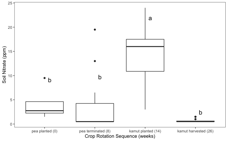
Figure 2) Soil nitrogen levels in ppm at each experimental point, from the original soil the peas were planted into, to the stage when peas were terminated, to the kamut planting stage, and finally at the end of the experiment when the kamut was harvested.
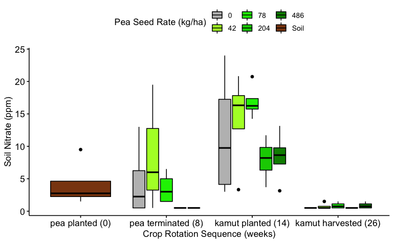
Figure 3) Soil nitrogen rates at each experimental point broken down further by pea seeding rate level.
The nitrogen rate was tracked in each individual box such that the effect of pea seeding rate could be assessed. In figure 3 we can see how pea seeding rates created varied levels of nitrate at each stage and especially the kamut planting stage. At this point it was assumed that most of the nitrogen tied up in the pea biomass had been broken down and made plant available. The N-level at kamut-planted stage has been corrected for nitrogen added by pea seed. Focusing in on the change in nitrate between when peas were seeded and when kamut seeded as seen in figure 4, we can see that as pea seeding rates rise the plant available nitrogen also rises. While the specific curve is somewhat unclear due to high variation; there does appear to be an optimum. There is weak evidence (p-value = 0.19) to support our model showing that soil nitrate reaches a peak at around 90 kg/ha pea seed rate and then starts declining as higher pea seeding rates become detrimental to pea growth through plant competition.
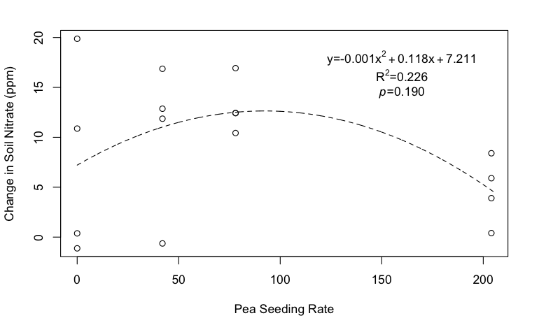
Figure 4) Change in soil nitrate in ppm between original pre-experiment soil and soil at the point of kamut planting when pea biomass had decomposed. Each point represents one enclosed planting box.
In the next stage of the experiment we tracked how kamut and pea seeding rates would affect final kamut yield. In figure five the curve shown fits a standard quadratic curve wherein the yield gains slow as seeding rates rise reaching a max yield around the maximum tested seeding rate of kamut. As kamut seeding rate rises we found strong evidence that overall kamut yield also rises reaching a peak level around a seeding rate of 120 kg/ha (p = 0.027). In figure 6 we see the affect of the pea seeding rate on kamut yield. In this situation we are tracking how the pea seeding rates affected the following crop’s yield. These results show a very similar trend to the soil nitrogen affects from pea seeding rate seen in figure 4. Here again we see weak evidence that pea seeding rate creates a maximum response in kamut yield around the 100kg/ha mark (p-value = 0.160). While repetitions were insufficient to show significance, we can nevertheless observe likely and predicted trends wherein low and high seeding rates are beyond optimum levels. These trends highlight the ability of a pea green manure crop to provide nitrogen to the following crop, while specific seeding rates of both the green manure and the cash crop are important in finding optimums. Moving to field experiments next we will predict site specific optimums.
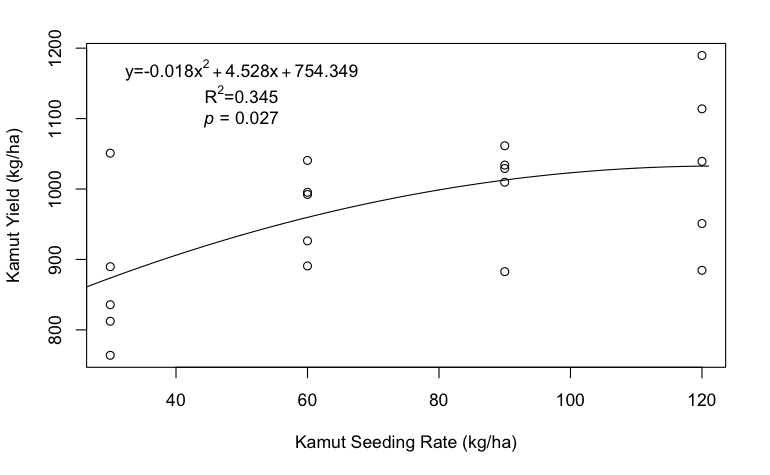
Figure 5) Kamut yield per garden box as a function of varied kamut seeding rates.
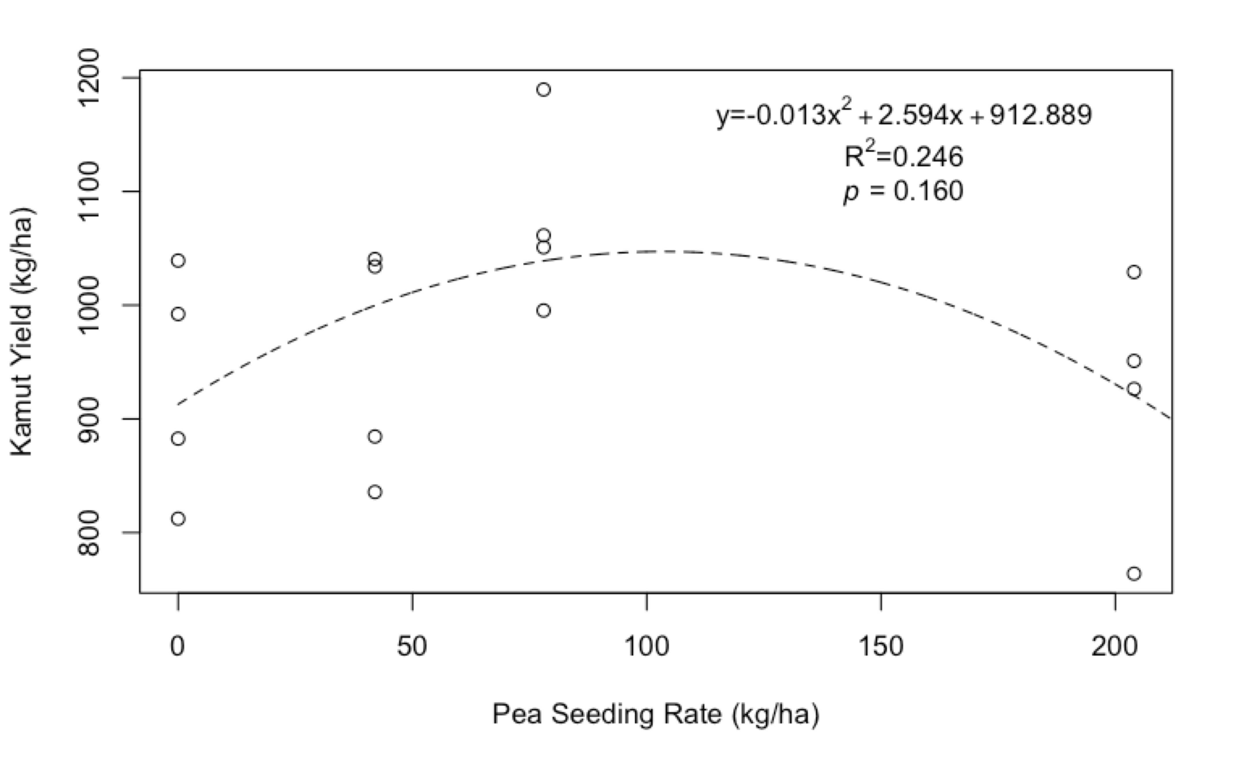
Figure 6) Kamut yield per garden box as a function of pea seeding rate.
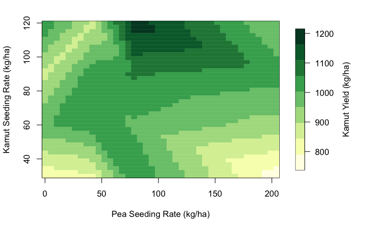
Figure 7) Kamut yield as a function of kamut seeding rate and underlying pea seeding rates. Highlighting the ability to find overlapping optimums.
By combining pea and kamut seeding rates we can determine overlapping seeding rates that lead to highest yielding combinations. As noted earlier optimum pea seeding rate appears around the 90-100kg/ha zone, and kamut yields respond to this as shown by the dark green area rising through the center of figure 7. Kamut yields tended to increase towards the higher rates tested, but appeared responsive to specific levels of pea seeding rates. We expect this trend then to be replicable for spatially variable field locations where each specific field space will be optimizable for both green manure and cash crop seeding rates. This was an important step in validating the proof of concept for our field experiments with varied pea and cereal crop seeding rates.
While the experimental conditions were able to mimic some Montana organic conditions, such as the sandy low N soil, the greenhouse otherwise provided excellent (unnatural) conditions for plant growth. Therefore this experiment is limited in the same way as all greenhouse experiments are limited in that they are not real conditions; there was no drought, no weeds, and perfect lighting conditions. Thus, while the first principle relationship between cover seeding density and following cash crop yield was established, it is now key to test this relationship in the field.
- ii & iii) On Farm Precision Experimentation of Seeding Rates and Harvest Yield and Model Results
RESULTS (of obj. ii & iii):
A list of final outcomes is shown in Tables 2 and 3. A specific example of the results is shown from farm A in compiled maps shown in Figure 8A-D. This is the same field as that shown in the methods section. From farm A we can see the output from simulations as generated using equation one from methods in the random forest model. These simulations predict yield and net return values based on three input scenarios. In the first scenario we include in the model farmer chosen single field rates (denoted as FRM in tables 2 and 3) for whichever input they experimented with; in the example shown this is pea green manure followed by the cash crop of barley. The second scenario shows optimized average rates (denoted OAV in tables 2 and 3) across the whole field based on maximizing net return using only one rate across the field. The third scenario (denoted VRT in tables 2 and 3) displays optimized rates of pea and barley varied across each cell of the field. The fourth panel of Figure 2 illustrates new randomized experimental rates that incorporate half of the field and the other half uses the newly discovered optimum rates.
In scenario one, shown in Figure 8A, farmer chosen rates of pea (90 lbs/ac) and barley (75 lbs/ac) are shown in panels 1 and 2, followed by yield and net return in panels 3 and 4. Due to low rainfall yields were relatively low on this field (11.25 bu/ac as seen in table 2). This effect is picked up in the model and when farmer chosen rates were simulated across the field the predicted yield was similarly low (10.98 bu/ac), generating a predicted net return of $62.21 per acre. The red and orange areas of the map denote the poorest performing areas of the field and we can see by comparing them to figure 1C, they tend to correspond to weedy areas of the field, and with figure 1A to higher areas of the field. Net returns were particularly low in those areas due presumably to weed competition and high elevation. These effects highlight the variability at play across the field.
Figure 8B shows simulated results from a scenario in which the farmer does not choose to vary rates across the whole field but rather chooses one optimum rate based on the results of our experiment. In this instance we note that the model has selected the lowest allowable rates for an optimized single rate. This again is likely an effect of the very dry year that was the last year of this experiment. Due to the lack of water lower plant densities perform better as they use less water from the field. By lowering the seeding rates our model predicts an increase in yield and due to decreased seed costs and increased yield a higher net return across the field, pushing net returns up to $72.60 per acre. These net returns come from both lowering seeding rates where they are not conducive to further yield growth, and from increasing yield by reducing intra-crop competition for water.
These gains are further improved upon as seen in figure 8C where variable rate of both pea and barley are allowed across the field. In this scenario we imagine the farmer planting specific varied rates of both cover and cash crop to maximize net return. We see further yield gains here as areas of the field that the model predicts can support higher plant densities are allowed to do so. In this way those prime areas of the field increase plant matter and consequent yield. Just as we saw in the greenhouse experiment where higher cover crop densities tended to produce higher cash crop yields so too here in certain parts of the field higher cover crop densities are predicted to improve cash crop outcomes. Through experimentation we have been able to pinpoint those areas and select them for increased plant densities in future seasons. Through this method net returns are maximized to a predicted $73.05/ac level, an increase of $10.84/ac above what the regular farmer used rates are predicted to have generated.
To compare these methods against each other statistically we used 21 years of historic economic data to understand how economic variation may favor one method over another. A compilation of these results for each farm is shown in Table 3. Following the mapped example to this table we see that the variable rate scenario, the scenario we predicted to generate the most outcome given economic realities of 2021, outcompetes both the farmer chosen rates, and the optimum average rates, in every year of economic conditions sampled. This same result was seen in farm B where the variable rate scenario fully outcompeted the other two scenarios 100% of the time. On farm C there was less certainty. While the variable rate scenario outcompeted the farmer chosen rates every time, the variable rate only outcompeted the optimum average scenario 67% of the time. This highlights that while variable rate is typically the best input rate strategy, the optimum average rate is a close second. Indeed on farms A, B, and C, the optimum average net return was considerably higher than the farmer chosen rate, and not very far behind the optimized variable rate method.
Farm D was the exception to the trends seen on the other farms. In this situation the farmer applied blood meal to experiment with the varied rates of nitrogen and their effect on their cash crop of spring wheat. While our goal as researchers was to learn about the variation in the field and optimize input rates, a broader result showed that blood meal had very little effect on the wheat yield. Due to its low effect on yield, any use of the product (which cost the farmer $1 per pound of nitrogen added per acre), reduced the farmers net return. In this instance the farmer learned a clear and valuable lesson about blood meal, that it was not worth their investment. Due to the experiment the farmer discontinued their use of the product and is exploring other organic nitrogen inputs instead. The result of that experiment is revealed in the comparison of variable rate to optimized average rate where the optimized variable input rate never outcompetes the optimized single rate since the model shows that the optimized rate of bloodmeal is zero on every grid cell of the field. The results of these experiments highlight the variability present across every field tested, and the ability to vary input seeding rates to maximize farmer net return.
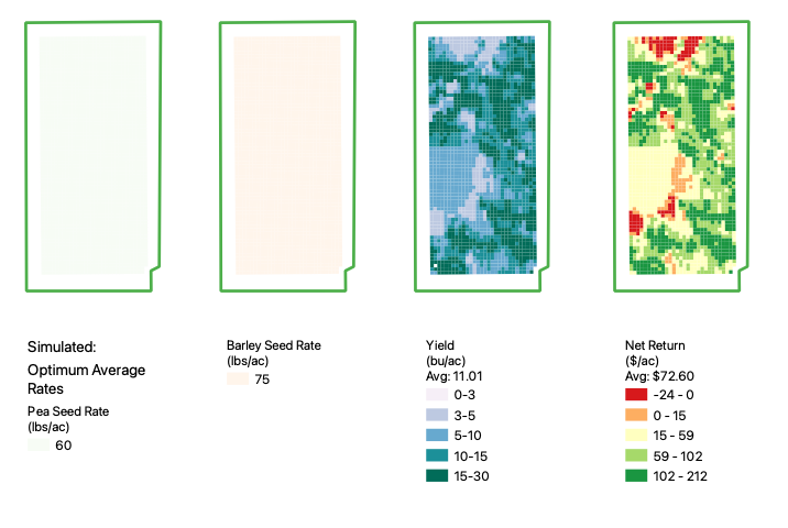
Figure 8A - 80 acre On Farm Precision Experimentation Field showing simulated results of applying farmer chosen rates, that is the rates the farmer would typically have seeded without experimentation. Panel 1) pea seeding rate, panel 2) barley seeding rate, panel 3) simulated yield from random forest model shown in equation 1, and panel 4) net return given seeding rates and simulated yield.
Figure 8B - 80 acre On Farm Precision Experimentation Field showing simulated results of applying optimum average rates, that is the single rates for pea (panel 1) and barley (panel 3) the model predicts would garner highest net return without varying rates across the field. Panel 3) simulated yield from random forest model shown in equation 1 given seeding rates shown, and panel 4) net return given these seeding rates and simulated yield.
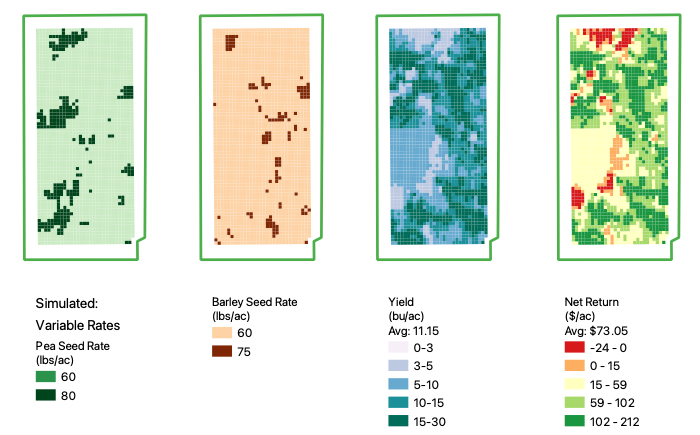
Figure 8C - 80 acre On Farm Precision Experimentation Field showing simulated results of applying optimum variable rates, that is the best rates for pea (panel 1) and barley (panel 3) the model predicts would garner highest net return given the option of varying rates in every cell across the field. Panel 3) simulated yield from random forest model shown in equation 1 given variable rate seeding rates, and panel 4) net return given these seeding rates and simulated yield.
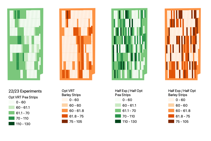
Figure 8D - 80 acre On Farm Precision Experimentation Field showing optimum variable rates given actual seeder capabilities in width (70’) and length given speed of variable rate change (240’); panel 1) optimum variable pea rates, 2) optimum variable barley rates, and in panels 3 and 4) half the strips are randomized such that experimentation can continue in the following season. These are the rates we would recommend for the farmer the following seasons this rotation repeats.
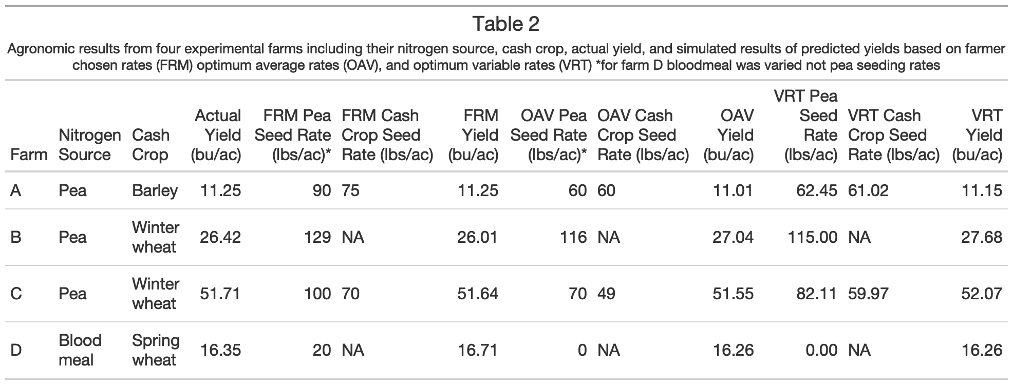
Table 2 – Agronomic results of experiments and simulations using three seeding strategies: farmer chosen rate, optimum average rate, and variable rate
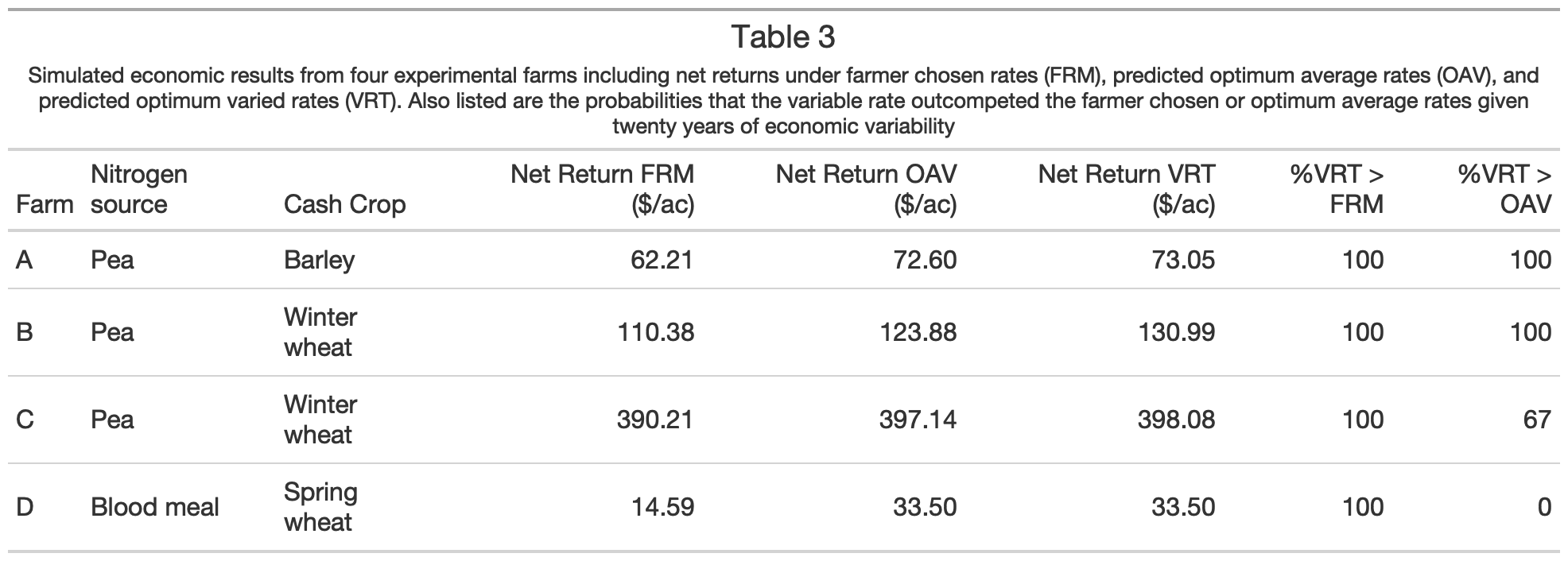
Table 3 – Economic results of experiments and simulations using three seeding strategies: farmer chosen rate, optimum average rate, and variable rate. Economic results include net return of each strategy and probability that variable rate seeding rates will outcompete the other two strategies over twenty years of economic variation.
- iv) OUTREACH results:
Research was shared through oral and poster presentations, in person when possible, and very often online after March 2020. One on one meetings were held with collaborator farmers at least semi-annually, to discuss results and future experimentation plans. Results were shared with students on university campuses, with crop consultants at workshops, with other researchers at research conferences, and with farmers at these same venues. A full list of presentations is shared below.
Publications:
Loewen, Sasha; Maxwell, Bruce (2021). On Farm Precision Experimentation in Organic Dryland Grain Production. OFE2021 Proceedings
Duff, H., Hegedus, P. B., Loewen, S., Bass, T., & Maxwell, B. D. (2022). Precision Agroecology. Sustainability, 14(1), 106.
Research outcomes
Education and Outreach
Participation summary:
Research was shared through oral and poster presentations, in person when possible, and very often online after March 2020. One on one meetings were held with collaborator farmers at least semi-annually, to discuss results and future experimentation plans. Results were shared with students on university campuses, with crop consultants at workshops, with other researchers at research conferences, and with farmers at these same venues. A full list of presentations is shared below.
PARA - Precision Ag Research Association - Dec. 3rd 2019 Great Falls MT, USA
-oral presentation
MOA - Montana Organic Association - Dec. 7th 2019 Bozeman MT, USA
-oral presentation
Crop Management School – January 7th 2020, Bozeman, MT, USA
-oral presentation
Sustainable Agriculture Guest Lecture – February 18th 2020 MSU, MT, USA
-oral presentation
Agroecology Class Guest Lecture – March 3rd 2020, MSU, MT, USA
-oral presentation
Prairie Organics Conference - March 5th 2020 Brandon, MB, Canada
-poster presentation
Soils n Crops Ag Conference - March 10th 2020 Saskatoon SK, Canada
-oral presentation
Department of Land Resources and Environmental Sciences student colloquium – April 29th 2020, online hosted by MSU
-oral presentation
Ecological Society of America – August 4th 2020 – online
-oral presentation
Precision Agriculture Research Association – November 30th 2020 - online
-oral presentation
Montana Organic Association – December 2nd 2020 - online
-oral presentation
Soils and Crops at University of Saskatchewan – March 16th 2021 – online
-oral presentation
Big Sky GeoCon by Montana Association of GIS Professionals – April 8th 2021 - online
-oral presentation
Montana State University Department of Land Resources and Environmental Sciences Colloquium – April 15th 2021 - online
-poster presentation
MontanaView Remote Sensing Fellowship Symposium, April 2021-online
-oral presentation
Farm Centric On Farm Experimentation 2021, October 2021 - online
-oral presentation
Montana Organic Association Annual Conference, December 2021 - online
-oral presentation
Precision Agriculture Research Association Annual Meeting, December 2021, online
-oral presentation
Montana Organic Association Student Summit, December 2021 - online
-oral presentation
Soils and Crops Conference, University of Saskatchewan, March 8, 2022 - online
-oral presentation
DIGICROP conference, University of Bonn and the AI Institute for Next Generation Food Systems, March 30, 2022 – online
-oral presentation